Filtering: From First-Order RC filters to Second-Order VCVS (voltage-controlled voltage source) filters

Wanting a filter means the input has some frequencies you regard as noise, and want them attenuated. A filter attenuates and phase shifts the input. It pretty much makes sense to talk about filters only in terms of linear circuits. (What can happen to frequencies after they pass through a nonlinear operator?) Here we will end up considering the 2-pole VCVS active filter applied the the problem of bandpass filter design.

In the next topic (Sampling) we will see LP filters applied to the problem of eliminating aliased frequencies due to sampling limitation.

¶ Reading: Handout on active filters, selected pages from Chpt 5 of Horowitz & Hill, The Art of Electronics (2nd Ed), Cambridge Univ Press (1989)

Filter specifications
Magnitude of response: Frequency range from passband, to stopband.
The spec will show what attenuation is required for which frequencies. Outside the attenuation range it is expected that the gain will be 1 (that would be ideal). The actual falloff of the filter, from pass to attenuation is determined the Order of the filter. (How many capacitors or inductors--energy storage elements--it has, number of poles in transfer function.) Sometimes the spec will require flatness in the passband.

Phase characteristics: If different frequencies are delayed different times then the output of the filter will not be a faithful version of the input. This lack of fidelity will be most clearly seen in response to step input, where overshoot and ringing may occur after filtering. Why does linear phase relationship mean that delay is constant? Suppose delay through the filter is 10 microseconds; 10 microseconds is a linearly increasing percentage of phase of increasing frequency. Thus linear phase is the goal, and Bessel filter is optimal for achieving linear phase.

Should the filter be adjustable? If so, there may be designs which allow a potentiometer to be changed, to change the frequency range.

A filter should also be insensitive to changes in R and C components due to heating or aging.

Filter types
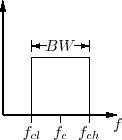
Ideal filter: step-like transitions: Impossible, but...Various filters will help you meet different specifications.
https://ccrma.stanford.edu/realsimple/aud_fb/What_Filter_Bank.html

Filter factor Q = fc/BW

Filter synthesis: Wonderful topic from years gone by in EE curriculum: place corner frequencies in a Laplace transform Zeros(s)/Poles(s) transfer function. An active filter involves the use of an op amp. For an active filter, consider Z(s) as the the feedback circuit, and P(s) as the source circuit in a negative gain summation amp.
Gain = -Z(s)/P(s)

HP = high pass filter, LP = low pass filter

Bandpass and notch filters
Combine HP and LP filters
two filters, LP, HP in series for bandpass,
band reject (notch) filter: two filters in parallel, summed for final output.

For the band reject, the cutoff for the LP filter < cutoff for HP filter.
The bandpass filter diagram is not quite complete: A unity gain voltage follower (UGVF) op amp is needed between the LP and HP filters to isolate the components in one filter from interacting with components in the other.

Equalizer: Suppose a set of 6 filters is designed to pass frequencies by the decade from 1 to 1,000,000 Hz (1-10, 10-100, 100-1000, etc). How should the six filters be combined into one output?

Butterworth filter
It's a maximally flat filter. In the passband the gain is optimally constant. The phase properties are not ideal, like Bessel, and the sharpness of cutoff is not as good as Chebychev. The Butterworth gain formula is

Chebychev Filter
Chebychev is maximally sharp in the transition from passband to stopband. The gain formula is
Notice the normalizing f/fc term is not taken to a power! and that the way to "unnormalize" the polynomial Cn is divide frequency by fc. Factor ε controls the amount of ripple in the passband. See Poularikis & Seely, p. 569. In the development in H&H page 275, the formulas are given in Hz, so 2*π is needed in the conversion to R and C in the VCVS circuit.

Chebychev polynomials:

Bessel filter: good time domain response.
A Bessel filter has maximally flat time delay, resulting in nearly linear phase. As frequency increases, a constant delay becomes an increasingly greater fraction of 360 degrees. If delay at different passband frequencies is not constant, then the resulting waveform will be distorted. Figure 5.14 in H&H, comparing Butterworth vs Bessel. See step response for example, Fig. 5.15.

VCVS circuit as a template for Bessel. Can use Table 5.2 for Bessel design.
The Gaussian filter: See Discussion in H&H, p. 272. Another filter with good phase characteristics.

Designing filters
Avoiding inductors
Inductors: RLC filters can provide excellent filter characteristics, and they are the analytic subject of RLC analysis in a Circuits class. BUT inductors are unwieldy, and have parasitic capacitance and conductance. Their real properties can degrade the performance of real filters. From H&H p. 266, on inductors: "They are often bulky and expensive, and they depart from the ideal by being 'lossy', .i.e., by having significant series resistance and other 'pathologies' such as nonlinearity, distributed winding capacitance, and susceptibility to magnetic pickup of interference." Goal: make good filters without the need for real inductors.

¶ The Op Amp chapter shows how to use a NIC (negative impedance converter) in a gyrator to convert "mathematically" a capacitor into an inductor.

Q (Quality factor) of an inductor or a filter
Q defines the sharpness of a bandpass filter, and is a term introduced in study of second order filters. Let β be the bandwidth of the filter and ω the center frequency: then

First order natural HP and LP filters
Recall from circuits class. one capacitor, one resistor, in the form of a voltage divider. Remember to use Radians/sec instead of Hertz in calculating component values. Shown below is an active LP filter. What is the gain at low frequency?

Always a bandpass: For the circuit below, say Cs are fixed, maybe C1 = C2 . Now say R1 = 10K and R2 = 1K, Question what kind of filter is represented? Consider that at low frequency a C is high Z, and at high freq, a C is low Z. At very low frequency the gain of the circuit is low, and at v. high freq the gain is also low, so the circuit must be bandpass.

Here is a derivation of the the transfer function, using j*w as the frequency variable:

If you reverse the resistors, and now make R1 = 1K and R2 = 10K, you have exactly the same shape gain vs freq curve! (with C1 = C2). Again a bandpass. (But if you put the parallel combination where Zs goes, and the series combination where Zf goes, what happens? You *can* come up with a band-reject filter.)

A matlab script to exercise the function above

Transfer function. In the analysis below we will find the ratio of output to input for a sinusoidal steady state input. Such a ratio is a transfer function commonly assumes a Laplace transform form: T(s). Assume we have one input only (each separate input deserves its own transfer function...superpostion can be used...). The initial conditions on the circuit (voltages on capacitors at t=0) will all be zero.

Analysis of VCVS active filter
Start with the Sallen & Key filter, Fig. 5.6.
See diagram below for voltage conventions.
Node analysis, with Vin V1, V2 and Vout = V2; second node has relationship between V1 and V2, solve for V2!

See matlab script for node admittance matrix solution to the Sallen and Key filter. Convention: current into node is negative, current out positive. The op amp must be treated as a voltage controlled voltage source (VCVS), and therefore is an asymmetric influence on the node admittance matrix. In the diagram below, node voltage V2 is at the V+ input of the op amp. Because there are 2 capacitors in the circuit, the filter is second order.

Have Matlab insert jwC in where Y2 and Y4 are, where w is the radial frequency in question.

A working version of the matlab VCVS code is shown at this link. The latest version is called VCVSfilt4.m and is found in the \work\fold23 folder. Notice that the actual output of the circuit is k*V2.

In Matlab abs calculates the magnitude of a complex number. If we were interested in phase angle, we would compute the tangent of (imag/real).

Remember, we are looking for the steady state sinusoidal response, a response which should depend only on the form of the transfer function, not the Laplace transform of any particular sinuosoid.

Example of a HP Bessel filter design using H&H tables:
Suppose you want to filter frequencies below 60 Hz. Meaning: You want a HP filter. You are given the criteria that at 0.5*the cutoff (30 Hz) the response is to be down by 10dB (0.3 attenuation). You are told to design a filter with linear phase. For construction, you have a variety of resistors, but only 0.3 :F capacitors to work with.

You decide to "design" a VCVS filter, using the information in Table 5.2 of H&H. You select a Bessel filter for good delay characteristics. Look on the graphs of page 276 H&H and see that at 2 x 60 Hz a 4th order filter is needed; second order doesn't have enough attenuation at 0.5x. You must use the 2x reading, since the graphs are for LP forms.

On page 275 H&H say, "To make a high-pass filter, use the high-pass configuration shown previously, with the [front end] Rs and Cs interchanged."
See Fig 5.16 for circuit. For the Bessel filters the normalizing factor fn must be inverted.
In table 5.2 you see that for 4 poles the Bessel terms are
K=1.084 and 1.759, and the fn terms are 1.432 and 1.606 respectively.
Invert the fn for 0.698 and 0.623.
For the first stage, if R = 10K, then (K-1)*R = 840 ohms
For the second stage, if R = 10K, then (K-1)*R = 7.6K ohms
For each stage, you can use R1 = R2 and C1 = C2 (Fig 5.16)
If we say C1 = 0.3:F, then R1 = 12.67K ohms
If we say C2 = 0.3:F, then R2 = 14.12K ohms

Analog vs Digital filters. Up to now we have assume filters are made with RC networks and supported by op amps. If your sinusoidal signal has been properly A-D converted and sent into LabVIEW there are an array of digital (software) filters which can mimic the effects of analog filters. In LabVIEW, on the Functions Menu see Analyze:Signal Processing:Filters for a set of Butterworth, Chebychev, etc digital filters. Filters in LabVIEW:

Summary List
¶ Filters for anti-aliasing
¶ Analog vs digital filters
¶ Active filters with op amps eliminate the need for inductors
¶ Specifications for filters: basic RC for first order LP and HP filters: gain, phase
¶ Making bandpass and band-reject filters from LP and HP blocks.
¶ Use of standard VCVS designs to meet specs.

Oct. 2003/08---------------------------------------------------------------
Misc notes below
Why filter? need for anti aliasing

the problem of inductors
passive vs active filters
optimal vs intuitive (RC) filters
first order filters: LP and HP
bandpass: LP and HP in series
Q: band-reject: LP and HP in parallel, converging on summation
Use of superposition
Distorted step response due to phase effects of filter
optimal higher order filters: Butterworth, Chebyshev, Bessel, Gaussian

Here in 123, we will consider the VCVS analog filter type, and learn to use tables, templates and software to meet filter specs as part of the Filter Quiz. Can use Matlab to generate exact spectrum

All LP filters will roll off at -20dB/decade per pole, when well above the cutoff frequency(ies). Or at 6 dB per octave.

Reading:
Oppenheim & Willsky, Signals and Systems, chapter 6, "Filtering" (1983)
Poularikas & Seely (URI), Signals and Systems, chapter 11, "Digital Filtering" (1985) See p. 568, Chebyshev filter form.

Bode plots: how to sketch gain and phase of a transfer function.
From EN52, you learned to make Bode plots of such transfer functions.
For specifying the filter characteristics of amplitude and phase vs freq. See page 704 of Nilsson (4th Ed)
A log-log plot, definition of dB considered: 20*log10(gain)
Real poles and zeros; complex poles and zeros.
First order plot: at w0=w the T(s) is -3dB, at 10x a pole is down -20dB, at 100x down -40dB, not a sharp skirt...