Consider a periodic function h(t), with period T. For any t:
Now say that we know that h(t) has no frequency component greater than N*f. In fact, for the sake of developing an example, say N=10.
Development of Sampling Theorem
Oct. 2003-04-08
The Sampling Theorem will be the single most important constraint you'll learn in instrumentation.
Here we want to move as efficiently as possible toward an understanding of the Sampling Theorem.
Periodic function described by sum of sines and cosines:
Consider a periodic function h(t), with period T. For any t: ![]() .
Let the fundamental frequency be
.
Let the fundamental frequency be ![]() .
.
Now say that we know that h(t) has no frequency component greater than N*f. In fact,
for the sake of developing an example, say N=10.
Exactly how we can say or know this maximum frequency constraint is a matter of some interest. Suffice it to say for now that an anti-aliasing LP filter may be used to help insure that h(t) is band-limited. More later about alias frequencies.
As described in a math course you've taken (example text: Thomas, Calculus
and Analytic Geometry, Addison-Wesley, 1960, pp 821-25), you can represent
h(t) exactly with the Fourier series:
![]()
where the n's are integers and there are (in this example) 21 coefficients, the
a's and the b's, to determine.
The first coefficient, a0, is the DC average of the
signal h(t): ![]() and can be calculated immediately, leaving the other 20.
and can be calculated immediately, leaving the other 20.
So at this point you can assume we are dealing with a periodic function of zero average.
Now we need to find the a's and b's. If you look in a calculus book, like Thomas,
you can find integral formulas of the sort:
![]() for
a 2*π period.
for
a 2*π period.
A more "brute force" computational way to find the a's and b's would be
to generate 20 independent equations by sampling. We can sample 20 times
during one period. If we sample over more than one period, we may not end up with
independent equations.
Each equation will be of the form ![]() where
m indexes the 20 samples.
where
m indexes the 20 samples.
The 20 equations can be formed into a 20x20 matrix C of coefficients times
a 20x1 column vector of unknowns = a 20x1 column vector of h(tm)
values.
 with
a solution
with
a solution 
The elements of C will be various sine and cosine terms in n, ω and
t.
Matlab will be able to invert matrix C in a matter of milliseconds.
So much for finding the a,b coefficients, which will be real, not
complex numbers. Each a,b pair says how much a particular frequency is weighted
in the summation leading to h(t). How should we combine an,
bn, for one measure of a particular frequency's
contribution? It turns out ![]() is a good choice. The Cn's represent
the spectrum of h(t).
is a good choice. The Cn's represent
the spectrum of h(t).
Now what about the spacing on the samples? If the spacing is uniform
there will be 2N segments of time, each segment the sample time (time between
samples). ![]() .
.
The maximum frequency in h(t) is![]() , therefore we have the Sampling Theorem:
, therefore we have the Sampling Theorem:
The sampling frequency must be greater than twice the highest frequency in
the input waveform in order for all frequencies in the input to be correctly
resolved. If the sampling criterion holds, then the input waveform can be exactly
reconstructed from it Fourier coefficients. Another way to say it: If
an input waveform is sampled at Fs, then the highest input frequency that can
be resolved without aliasing is Fs/2.
Another statement of the Sampling Theorem, from A. V. Oppenheim
and A. S. Willsky, Signals and Systems, 2nd Ed. Prentice-Hall (1996)
p. 518:
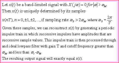
Terminology: The sampling frequency of a particular situation, which may exceed by quite a bit the maximum frequency in the signal, is the Nyquist frequency. Twice the maximum frequency of the signal is called the Nyquist rate, and is the minimum sampling rate that can resolve the signal. (O&W, 1st Ed, p. 519)
Smallest frequency difference to be resolved
Example: Imagine that sampling goes on for one second, at a rate of 20
Hz. 20 samples will be taken, and 10 frequency spectrum coefficients can be
computed. Since the maximum resolvable frequency is 10 Hz, the 10 coefficients
must represent frequencies spaced 1Hz apart. 1Hz is therefore the minimum resolvable
frequency difference. What if the sampling goes on for 2 seconds, at 20 Hz?
Then there will be 40 samples for 20 frequencies, still with a max of 10 Hz
and therefore a 0.5Hz difference between steps in the spectrum. It should begin
to make sense to you that, for a constant sample rate, as the sampling
time increases, the frequency difference between intervals in the spectrum
decreases. The relationship is ![]()
Suppose you want to resolve manual frequency of knob rotation to the nearest
0.1Hz. How long will the subject have to turn the knob back and forth while
you sample? 10 seconds. If you sample and audio signal at 40000 Hz rate for
0.1 seconds, the spacing on the spectrum will be what? 10 Hz.
How frequently does the FFT display on your digital scope update?
Discrete Fourier Transform Notation from C. Williams, Designing Digital
Filters, Prentice-Hall (1986) p. 262. It is worth inspecting the
formula that shows how Fourier coefficients H are computed in a computer:
The DFT is ![]()
where both i and k range from 0 to N-1 and j is the imaginary number. The sampled
values are in the list hk.
The H are usually complex numbers, and their magnitudes must be taken to find
the Power Spectrum.
The inverse DFT is ![]()
where hk is a list of numbers brought in by sampling
a waveform: Or, in the case of the DFT, a list of numbers that reconstruct a
waveform from its spectrum H.
A standard reference is A.V. Oppenheim & S. Willsky,
Signals and Systems, 2nd Ed., Prentice-Hall (1997). See chapter 3, "Fourier
Series Representation of Periodic Signals." Much of the development in their
chapter uses the Euler identity, ![]() ,
where j is the imaginary number.
,
where j is the imaginary number.
Williams points out (chpt 2) that the complex exponential is an eigenfunction for digital filters and therefore better, mathematically, for demonstrating properties of digital filters.
In fact, a faster algorithm, the Fast Fourier Transform (FFT), is normally computed, for example, in LabVIEW or MATLAB on in the math feature of the HP 54622A digital scope.
Mathematically, the FFT receives as input a vector of real numbers that represent evenly spaced samples in time, and returns as output a vector of the same size, likely of complex numbers, that represent coefficients of a spectrum. The "user" must be able to interpret what the frequency spacing is on the output vector. The "power spectrum" is the magnitude of the complex numbers.
EXAMPLE: In the command line of MATLAB,
type vec = [ 1 2 3 4 3 2 -1 -2 0 1 2 -1 -3 -5 -2 1];
in MATLAB notation: 16 data points.
type vec_out = fft(vec); to generate
a list of 16 complex numbers.
type pwer = abs(vec_out); to find the magnitudes of
the complex numbers.
type plot( [0:15], pwer) to generate the plot below:
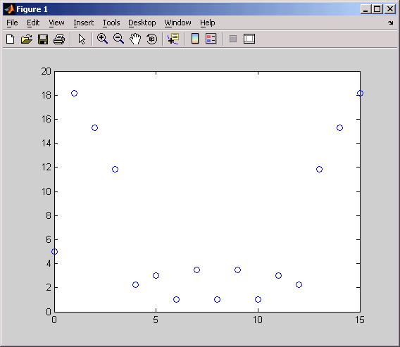
Notice the plot is symmetic about "frequency" 8, except for the 0
data point. The 0 frequency data point is the DC average of vec * 16 = 5. The
data from 8 above is a mirror image of the true spectrum, represented by the
lower half of the plot.
Aliased frequencies:
The Sampling Theorem says that input waveforms with frequencies below the half
sampling rate can be reconstructed exactly. Frequencies above the half the sampling
rate become aliased as lower frequencies: For frequencies just above the half
the sampling rate, up to the sampling rate, the aliased frequency falias
= fnyq-|factual - fnyq|,
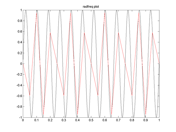
a kind of mirror-image result. See Matlab example (alias03.m
file) below, where the waveform to be sampled is in gray. It is a
12 Hz sinewave and would therefore require greater than 24 Hz sampling rate
to preserve the correct frequency in reconstruction. The red line is the result
of sampling at 20 Hz; the alias is therefore 10- abs(10-12) = 8 Hz.
An input at exactly the sampling rate is "standing still", as you will
see in the strobe demo.
The graph below shows the triangle waveform for aliased frequencies greater than Fsamp.
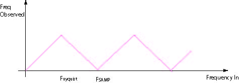
The F-obs waveform is periodic on F-samp. Here's an attempt to formalize the triangle
waveform: Say f-act = actual input frequency:
Divide f-act by f-nyq and express the answer as integer + remainder: ![]()
next let B = INT mod 2 (even = 0, odd = 1)
then f-obs = REM + B * (f-nyq - 2 * REM)
Demo of aliasing with strobe light. In a darkened room aim a strobe
light at a fan. The fan's 3 blades will have the number"123" written
in different colors. Think of the strobe frequency as the sampling frequency.
One thing we would like to know: At what Hz are the fan blades rotating? (the
fan has SLO MED FAST settings)
Example from the
web.
If we can set the strobe to the same rate as the fan rotation frequency, then the fan blades will appear to stand still and the one blade with "123" will be visible. The fan rotation frequency will be aliased to 0Hz because the sampling rate will equal the input frequency rate.
But if the strobe is at exactly half the fan frequency, the blades will also stop! Why? Because now the "input" of fan frequency is 2x the sampling rate, another zero point on the alias figure above. How can you make sure the strobe freq is set at the fan frequency? One way: bring the strobe down from an obviously high frequency, then the FIRST time the blades "stop" so 3 blades are seen, must be the correct frequency.
What do you see if the strobe frequency is at 2x the fan frequency?
Notice that when the strobe is set at the fan frequency slight changes in the strobe frequency up or down cause the fan blades to rotate slowly either CW or CCW. The slow rotations may be at the same slow frequencies, but in different directions: What does this phase difference mean for interpretation of aliasing?
So: Aliased frequencies may be bad news for electrical spectrum analyzers, but for mechanical rotation they can be a helpful measurement.
About the strobe: General Radio 1531A, from 1971. The circuit used to drive
the 10 microseconds of the Xenon flash tube is similar to a defibrillator. Charging
a capacitor up to several hundred volts. Why no new strobe models on the market?
Fear of lawsuits about epilepsy, or the high voltage?
Digital Filters
The inputs to a digital filter come from a tapped delay line (TDL). The delay
time is the sampling time. The number of input taps to the filter is a measure of
the filter's size. An example from
http://www-ccrma.stanford.edu/~jos/waveguide/Example_Tapped_Delay_Line.html
is shown below, where x(n) is the sampled input waveform to be tapped and filtered.
The notation![]() means "delay of δ t".
means "delay of δ t".
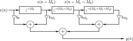
Normally the TDL is in software. The taps pass through coefficients (bMi above) to a sum-of-products, whose output is the filter output, in the case above, y(n). Designing a digital filter means selecting the proper coefficients. If the coefficients are all positive some kind of LP filter results. If the coefficients alternate in sign some kind of HP filter results. Here is a website that reviews sum-of-product filter design, and here is one that generates C code digital filters of various types.
Cutoff frequency for anti-aliasing LP filter.
Example: Suppose there is noise at all frequencies (white noise), but that your
signal has information only below 1000 Hz. What would be a reasonable sampling
rate and what should be the cutoff frequency for the anti-aliasing filter?
Placement of anti-aliasing filter: BEFORE A-D converter! (not feasible to be a software filter).
Approximation due to sampling: See lecture notes on A-D conversion
2008-09 see jdd/Reconstruct08b.m
[FofT, FofT_cont, tim_sine] = Recnstrct08b(inp_mde, snsoid_type, spc_mde, calc_mde,
wind_flg, samp_num, sine_max)
to investigate reconstruction and FFT coefficients.