3. Kinematics
3.1 Basic Assumptions
Continuum
mechanics is a combination of mathematics and physical laws that approximate
the large-scale behavior of matter that is subjected to mechanical
loading. It is a generalization of
Newtonian particle dynamics, and starts with the same physical assumptions
inherent to Newtonian mechanics; and adds further assumptions that describe the
structure of matter. Specifically:
 The Newtonian reference frame: In classical continuum mechanics, the world is idealized
as a three dimensional Euclidean space (a vector space consisting of all triads
of real numbers ). A point in space is identified by a unique
set of three real numbers. A Euclidean
space is endowed with a metric, which
defines the distance between points: . Vectors can be expressed as components in a basis
- of mutually perpendicular unit vectors. Physical quantities such as force, velocity,
acceleration are expressed as vectors in this space. A Cartesian
Coordinate Frame is a fixed point O together with a basis. A Newtonian
reference frame is a particular choice of Cartesian coordinate frame in
which Newton’s laws of motion hold.
The Newtonian reference frame: In classical continuum mechanics, the world is idealized
as a three dimensional Euclidean space (a vector space consisting of all triads
of real numbers ). A point in space is identified by a unique
set of three real numbers. A Euclidean
space is endowed with a metric, which
defines the distance between points: . Vectors can be expressed as components in a basis
- of mutually perpendicular unit vectors. Physical quantities such as force, velocity,
acceleration are expressed as vectors in this space. A Cartesian
Coordinate Frame is a fixed point O together with a basis. A Newtonian
reference frame is a particular choice of Cartesian coordinate frame in
which Newton’s laws of motion hold.
 The Continuum: Matter is idealized as a continuum, which has two properties: (i) it is infinitely divisible
(you can subdivide some region of the solid as many times as you wish); and
(ii) it is locally homogeneous in other words if you subdivide it
sufficiently many times, all sub-divisions have identical properties (eg mass
density). A continuum can be thought of
as an infinite set of vanishingly small particles, connected together.
The Continuum: Matter is idealized as a continuum, which has two properties: (i) it is infinitely divisible
(you can subdivide some region of the solid as many times as you wish); and
(ii) it is locally homogeneous in other words if you subdivide it
sufficiently many times, all sub-divisions have identical properties (eg mass
density). A continuum can be thought of
as an infinite set of vanishingly small particles, connected together.
Both
the existence of a Newtonian reference frame, and the concept of a continuum,
are mathematical idealizations.
Experimental evidence suggest that the laws of motion based on these
assumptions accurately approximate the behavior of most solid and fluid
materials at length scales of order mm-km or so in engineering
applications. In some cases continuum
models can also approximate behavior at much shorter length scales (for volumes
of material containing a few 1000 atoms), but models at these length scales
often require different relations between internal forces deformation measures
in the solid to those used to model larger volumes.
3.2 Reference and
deformed configuration of a solid
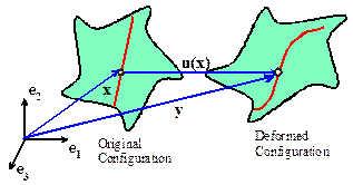
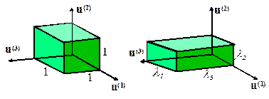
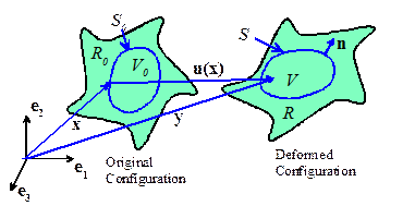
The configuration of a solid is a region of space occupied (filled) by
the solid. When we describe motion, we
normally choose some convenient configuration of the solid to use as reference - this is often the initial, undeformed solid,
but it can be any convenient region that could be occupied by the solid. The material changes its shape under the
action of external loads, and at some time t
occupies a new region which is called the deformed or current
configuration of the solid.
For some applications (fluids,
problems with growth or evolving microstructures) a fixed reference
configuration can’t be identified in this case we usually use the deformed
material as the reference configuration.
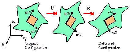
Mathematically, we describe a deformation as a 1:1 mapping which
transforms points from the reference configuration of a solid to the deformed
configuration. Specifically, let be three numbers specifying the position of
some point in the undeformed solid (these could be the three components of
position vector in a Cartesian coordinate system, or they could be a more
general ccoordinate system, such as polar coordinates). As the solid deforms, each the values of the
coordinates change to different numbers.
We can write this in general form as . This is called a deformation mapping.
To be a physically admissible
deformation
(i) The
coordinates must specify positions in a Newtonian reference frame. This means that it must be possible to find
some coordinate transformation ,
such that are components in an orthogonal basis, which
is taken to be ‘stationary’ in the sense of Newtonian dynamics.
(ii) The
functions must be 1:1 on the full set of real numbers;
and must be invertible
(iii) must be continuous and continuously
differentiable (we occasionally relax these two assumptions, but this has to be
dealt with on a case-by-case basis)
(iv) The mapping must satisfy .
To begin with, we will describe
all motions and deformations by expressing positions of points in both undeformed
and deformed solids as components in a Cartesian reference frame (which is also
taken to be an inertial frame). Thus will denote components of the position vector
of a materal particle before deformation, and will be components of its position vector after
deformation.
3.3 The Displacement and Velocity
Fields
The displacement vector u(x,t) describes the motion of each point in the solid. To make this
precise, visualize a solid deforming under external loads. Every point in the solid moves as the load is
applied: for example, a point at position x
in the undeformed solid might move to a new position y at time t. The displacement vector is defined as
We could also express this formula using index notation, as
Here, the subscript i has values 1,2, or 3, and (for example) represents the three Cartesian components of
the vector y.
The displacement field completely specifies the change
in shape of the solid. The velocity field
would describe its motion, as
We also define the acceleration
field
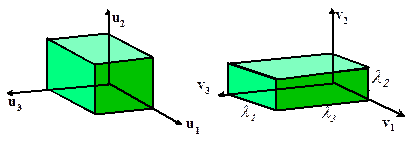
Examples
of some simple deformations
|
Volume
preserving uniaxial extension
|
|
|
|
Simple shear
|
|
|
|
Rigid rotation through angle about axis
|

|
|
General rigid rotation about the origin
where R must satisfy ,
det(R)>0. (i.e. R is proper orthogonal). I is the identity tensor with components
Alternatively, a rigid rotation through angle (with right hand screw convention) about an
axis through the origin that is parallel to a unit vector n can be written as
The components of R are
thus
where is the permutation
symbol, satisfying
|
|
|
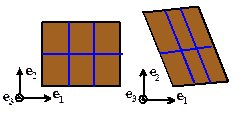
General homogeneous deformation
or
where are constants.
The physical significance of a homogeneous
deformation is that all straight lines in the solid remain straight under the
deformation. Thus, every point in the
solid experiences the same shape change.
All the deformations listed above are examples of homogeneous
deformations.
|
|
3.4 Eulerian and Lagrangian descriptions of motion and deformation.
The displacement and
velocity are vector valued functions.
In any application, we have a choice of writing the vectors as functions
of the position of material particles before deformation
This is
called the lagrangean description of
motion. It is usually the easiest way to
visualize a deformation.
But in
some applications (eg fluid flow problems, where it’s hard to identify a
reference configuration) it is preferable to write the displacement, velocity
and acceleration vectors as functions of the deformed position of particles.
These express displacement,
velocity and displacement as functions of a particular point in space
(visualize describing air flow, for example).
This is called the Eulerian
description of motion. Of course the functions of and are not the same we just run out of symbols if we introduce
different variables in the Lagrangian and Eulerian descriptions.
The
relationships between displacement, velocity, and acceleration are somewhat
more complicated in the Eulerian description.
In the laws of motion, we normally are interested in the velocity and
acceleration of a particular material particle, rather the rate of change of
displacement and velocity at a particular point in space. When computing the time derivatives, it is
necessary to take into account that is a function of time. Thus, displacement, velocity and acceleration
are related by
You can derive these results
by a simple application of the chain rule.
3.5 The Displacement gradient and
Deformation gradient tensors
These
quantities are defined by
Displacement
Gradient Tensor: is a tensor with components
Deformation
Gradient Tensor:
where I is
the identity tensor, with components described by the Kronekor delta symbol:
and represents the gradient operator. Formally,
the gradient of a vector field u(x) is defined so that
but in practice the component formula is more useful.
Note also that
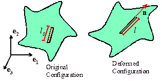
 The concepts of displacement gradient and deformation
gradient are introduced to quantify the change in shape of infinitesimal line
elements in a solid body. To see this, imagine drawing a straight line on the undeformed
configuration of a solid, as shown in the figure. The line would be mapped to a smooth curve on
the deformed configuration. However,
suppose we focus attention on a line segment dx, much shorter than the radius of curvature of this curve, as
shown. The segment would be straight in
the undeformed configuration, and would also be (almost) straight in the
deformed configuration. Thus, no matter
how complex a deformation we impose on a solid, infinitesimal line segments are
merely stretched and rotated by a deformation.The infinitesimal line segments dx and dy are related by
The concepts of displacement gradient and deformation
gradient are introduced to quantify the change in shape of infinitesimal line
elements in a solid body. To see this, imagine drawing a straight line on the undeformed
configuration of a solid, as shown in the figure. The line would be mapped to a smooth curve on
the deformed configuration. However,
suppose we focus attention on a line segment dx, much shorter than the radius of curvature of this curve, as
shown. The segment would be straight in
the undeformed configuration, and would also be (almost) straight in the
deformed configuration. Thus, no matter
how complex a deformation we impose on a solid, infinitesimal line segments are
merely stretched and rotated by a deformation.The infinitesimal line segments dx and dy are related by
Written
out as a matrix equation, we have
To derive this result, consider an infinitesimal line
element dx in a deforming
solid. When the solid is deformed, this
line element is stretched and rotated to a deformed line element dy. If
we know the displacement field in the solid, we can compute dy=[x+dx+u(x+dx)]-[x+u(x)] from the
position vectors of its two end points
Expand
as a Taylor
series
so
that
We
identify the term in parentheses as the deformation gradient, so
The inverse
of the deformation gradient arises in many calculations. It is defined through
or
alternatively
3.6 Deformation gradient resulting
from two successive deformations
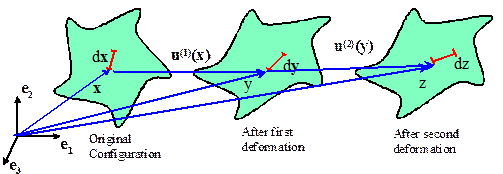
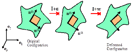
Suppose that
two successive deformations are applied to a solid, as shown. Let
map infinitesimal line elements from the original
configuration to the first deformed shape, and from the first deformed shape to
the second, respectively, with
The
deformation gradient that maps infinitesimal line elements from the original
configuration directly to the second deformed shape then follows as
Thus, the
cumulative deformation gradient due to two successive deformations follows by
multiplying their individual deformation gradients.
To see this,
write the cumulative mapping as and apply the chain rule
3.7 The Jacobian of the deformation
gradient change of volume
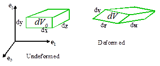 The Jacobian is defined as
It is a measure of the volume change produced by a
deformation. To see this, consider the
infinitessimal volume element shown with sides dx, dy, and dz in the figure above. The original
volume of the element is
Here,
is the permutation symbol. The element is
mapped to a paralellepiped with sides dr, dv, and dw with volume given by
Recall
that
so
that
Recall
that
so
that
Hence
Observe
that
For any physically admissible deformation, the
volume of the deformed element must be positive (no matter how much you deform
a solid, you can’t make material disappear).
Therefore, all physically admissible displacement fields must satisfy J>0
If a material is incompressible, its volume remains constant. This requires J=1.
If the mass
density of the material at a point in the undeformed solid is , its mass density in the deformed solid
is
Derivatives
of J. When working with constitutive
equations, it is occasionally necessary to evaluate derivatives of J with respect to the components of F.
The following result (which can be proved e.g. by expanding the Jacobian
using index notation see HW1, problem 7, eg) is extremely useful
 3.8 Transformation
of internal surface area elements
3.8 Transformation
of internal surface area elements
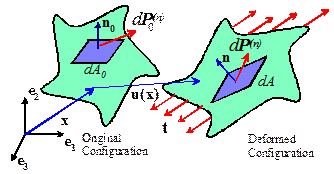
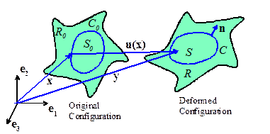
When we deal with internal forces in a solid, we need
to work with forces acting on internal surfaces in a solid. An important question arises in this
treatment: if we identify an element of area with normal in the reference configuration, and then what
are the area of and normal of this area element in the deformed solid?
The
two are related through
To
see this,
1. let be two infinitesimal material fibers with
different orientations at some point in the reference configuration. These fibers bound a parallelapiped with area
and normal
2. The vectors map to , in the deformed solid
3. In the deformed solid the area element is thus
4. Recall the identity - so
3.8 The Lagrange strain tensor
 The Lagrange strain tensor is defined as
The components of Lagrange strain can also be
expressed in terms of the displacement gradient as
The Lagrange strain tensor quantifies the changes in
length of a material fiber, and angles between pairs of fibers in a deformable
solid. It is used in calculations where
large shape changes are expected.
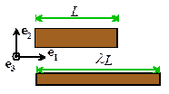
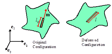
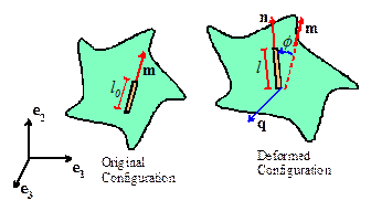
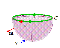
To visualize the physical significance of E, suppose we mark out an imaginary
tensile specimen with (very short) length on our deforming solid, as shown in the
picture. The orientation of the specimen is arbitrary, and is specified by a
unit vector m, with components . Upon deformation, the specimen increases in
length to .
Define the strain of the specimen as
Note that this definition of strain is similar to the
definition you are familiar with, but contains an
additional term. The additional term is
negligible for small .
Given the Lagrange strain components ,
the strain of the specimen may be computed from
We
proceed to derive this result. Note that
is an infinitesimal vector with length and orientation
of our undeformed specimen. From the
preceding section, this vector is stretched and rotated to
The length of the deformed specimen is equal to the
length of dy, so we see that
Hence, the strain for our line element is
giving
the results stated.
3.9 The Eulerian strain tensor
The
Eulerian strain tensor is defined as
Its physical significance is similar to the Lagrange
strain tensor, except that it enables you to compute the strain of an
infinitesimal line element from its orientation after deformation.
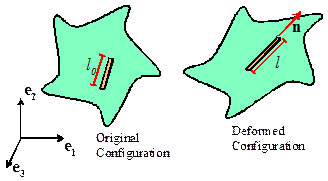
Specifically, suppose that n denotes a unit vector parallel to the deformed material fiber, as
shown in the picture. Then
The
proof is left as an exercise.
3.10 The Infinitesimal strain tensor
The
infinitesimal strain tensor is defined as
where
u is the displacement vector. Written out in full
The
infinitesimal strain tensor is an approximate
deformation measure, which is only valid for small shape changes. It
is more convenient than the Lagrange or Eulerian strain, because it is linear.
Specifically, suppose the deformation gradients are
small, so that all .
Then the Lagrange strain tensor is
so the infinitesimal strain approximates the Lagrange
strain. You can show that it also
approximates the Eulerian strain with the same accuracy.
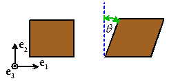
Properties of the infinitesimal strain
tensor
For small strains, the engineering strain of
an infinitesimal fiber aligned with a unit vector m can be estimated as
Note that
(see below for more details)
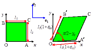 The infinitesimal strain tensor is closely
related to the strain matrix introduced in elementary strength of materials
courses. For example, the physical
significance of the (2 dimensional) strain matrix
The infinitesimal strain tensor is closely
related to the strain matrix introduced in elementary strength of materials
courses. For example, the physical
significance of the (2 dimensional) strain matrix
is illustrated in the
figure.
To relate this to the infintesimal strain tensor, let be a Cartesian basis, with parallel to x and parallel to y as shown. Let denote the components of the infinitesimal
strain tensor in this basis. Then
3.11
Engineering shear strains
For a general strain tensor (which could be any of ,
or ,
among others), the diagonal strain components are known as `direct’ strains, while the off
diagonal terms are known as ‘shear strains’
The shear strains are sometimes reported as
‘Engineering Shear Strains’ which are related to the formal definition by a
factor of 2 i.e.
This factor of 2 is an endless source of
confusion. Whenever someone reports
shear strain to you, be sure to check which definition they are using. In particular, many commercial finite element
codes output engineering shear strains.
3.12 Decomposition of infinitesimal strain
into volumetric and deviatoric parts
The
volumetric infinitesimal strain is
defined as
The
deviatoric infinitesimal strain is
defined as
The
volumetric strain is a measure of volume changes, and for small strains is
related to the Jacobian of the deformation gradient by . To see this, recall that
The
deviatioric strain is a measure of shear deformation (shear deformation
involves no volume change).
3.13 The Infinitesimal rotation tensor
The
infinitesimal rotation tensor is defined as
Written
out as a matrix, the components of are
Observe
that is skew
symmetric: .
A skew tensor represents a rotation through a small
angle. Specifically, the operation rotates the infinitesimal line element through a small angle about an axis parallel to the unit vector . (A skew tensor also sometimes represents an
angular velocity).
To visualize the significance of ,
consider the behavior of an imaginary, infinitesimal, tensile specimen embedded
in a deforming solid. The specimen is
stretched, and then rotated through an angle about some axis q. If the displacement
gradients are small, then .
The rotation of the specimen depends on its original
orientation, represented by the unit vector m. One can show (although
one would rather not do all the algebra) that represents the average rotation, over all possible orientations of m, of material fibers passing through a
point.
As
a final remark, we note that a general deformation can always be decomposed
into an infinitesimal strain and rotation
Physically,
this sum of and can be regarded as representing two successive
deformations a small strain, followed by a rotation, in the
sense that
first
stretches the infinitesimal line element, then rotates it.
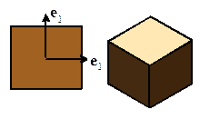
3.14 Principal values and directions of
the infinitesimal strain tensor
The three principal values and directions of the infinitesimal strain tensor satisfy
Clearly, and are the eigenvalues and eigenvectors of . There are three principal strains and three
principal directions, which are always mutually perpendicular.
Their significance can be visualized as follows.
1. Note that the decomposition can be visualized as a small strain, followed
by a small rigid rotation, as shown in the picture.
2. The formula indicates that a vector n is mapped to another, parallel vector
by the strain.
3. Thus, if you draw a small cube with its faces
perpendicular to on the undeformed solid, this cube will be
stretched perpendicular to each face, with a fractional increase in length . The faces remain perpendicular to after deformation.
4. Finally, w
rotates the small cube through a small angle onto its configuration in the
deformed solid.
3.15
Strain Equations of Compatibility for infinitesimal strains
It
is sometimes necessary to invert the
relations between strain and displacement that is to say, given the strain field, to
compute the displacements. In this section, we outline how this is done, for
the special case of infinitesimal
deformations.
For infinitesimal motions the
relation between strain and displacement is
Given
the six strain components (six, since ) we wish to determine the three displacement
components .
First, note that you can never completely recover the displacement field that
gives rise to a particular strain field.
Any rigid motion produces no strain, so the displacements can only be
completely determined if there is some additional information (besides the
strain) that will tell you how much the solid has rotated and translated. However, integrating the strain field can
tell you the displacement field to within an arbitrary rigid motion.
Second,
we need to be sure that the strain-displacement relations can be integrated at
all. The strain is a symmetric second
order tensor field, but not all symmetric second order tensor fields can be
strain fields. The strain-displacement relations amount to a system of six
scalar differential equations for the three displacement components ui.
To be integrable, the strains
must satisfy the compatibility
conditions, which may be expressed as
Or, equivalently
Or, once more equivalently
It
is easy to show that all strain fields must satisfy these conditions - you simply need to substitute for the strains
in terms of displacements and show that the appropriate equation is satisfied. For example,
and similarly for the other
expressions.
Not that for planar
problems for which all of these compatibility equations are
satisfied trivially, with the exception of the first:
It
can be shown that
(i) If the
strains do not satisfy the equations of compatibility, then a displacement
vector can not be integrated from the strains.
(ii) If the strains satisfy the compatibility
equations, and the solid simply connected
(i.e. it contains no holes that go all the way through its thickness), then
a displacement vector can be integrated from the strains.
(iii) If the solid is not simply connected, a
displacement vector can be calculated, but it may not be single valued i.e. you may get different solutions depending
on how the path of integration encircles the holes.
Now,
let us return to the question posed at the beginning of this section. Given the strains, how do we compute the
displacements?
2D strain fields
For
2D (plane stress or plane strain) the procedure is quite simple and is best
illustrated by working through a specific case
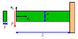
As
a representative example, we will use the strain field in a 2D (plane stress)
cantilever beam with Young’s modulus E
and Poisson’s ratio loaded at one end by a force P. The beam has a rectangular
cross-section with height 2a and
out-of-plane width b. We will show
later (Sect 5.2.4) that the strain field in the beam is
We first check that the
strain is compatible. For 2D problems
this requires
which is clearly satisfied
in this case.
For
a 2D problem we only need to determine and such that
.
The first two of these give
We
can integrate the first equation with respect to and the second equation with respect to to get
where
and are two functions of and ,
respectively, which are yet to be determined.
We can find these functions by substituting the formulas for and into the expression for shear strain
We can re-write this as
The
two terms in parentheses are functions of and ,
respectively. Since the left hand side
must vanish for all values of and ,
this means that
where is an arbitrary constant. We can now integrate these expressions to see
that
where c and d are two more
arbitrary constants. Finally, the displacement field follows as
The
three arbitrary constants ,
c and d can be seen to represent a small rigid rotation through angle about the axis, together with a displacement (c,d) parallel to axes, respectively.
 3D strain
fields
3D strain
fields
For
a general, three dimensional field a more formal procedure is required. Since
the strains are the derivatives of the displacement field, so you might guess
that we compute the displacements by integrating the strains. This is more or less correct. The general procedure is outlined below.
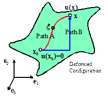
We
first pick a point in the solid, and arbitrarily say that the
displacement at is zero, and also take the rotation of the
solid at to be zero. Then, we can compute the displacements
at any other point x in the solid,
by integrating the strains along any convenient path. In a simply connected solid, it doesn’t
matter what path you pick.
Actually,
you don’t exactly integrate the strains instead, you must evaluate the following
integral
where
Here,
are the components of the position vector at
the point where we are computing the displacements, and are the components of the position vector of a point somewhere along the path of
integration. The fact that the integral is path-independent (in a simply
connected solid) is guaranteed by the compatibility condition. Evaluating this integral in practice can be
quite painful, but fortunately almost all cases where we need to integrate
strains to get displacement turn out to be two-dimensional.
3.16 Cauchy-Green Deformation Tensors
There
are two Cauchy-Green deformation tensors defined through
The
Right Cauchy Green Deformation Tensor
The
Left Cauchy Green Deformation Tensor
They are called `left’ and `right’ tensors because of
their relation to the `left’ and ‘right’ stretch tensors defined below. They can be regarded as quantifying the
squared length of infinitesimal fibers in the deformed configuration, by noting
that if a material fiber in the undeformed solid is stretched and
rotated to in the deformed solid, then
3.17 Rotation tensor, and Left and Right
Stretch Tensors
The
definitions of these quantities are
The
Right Stretch Tensor
The
Left Stretch Tensor
The
Rotation Tensor
To calculate these quantities you need to remember how
to calculate the square root of a matrix.
For example, to calculate the square root of C, you must
1. Calculate the eigenvalues of C we will call these ,
with n=1,2,3. Since C
and B are both symmetric and
positive definite, the eigenvalues are all positive real numbers, and therefore
their square roots are also positive real numbers.
2. Calculate the eigenvectors of C and normalize them so they
have unit magnitude. We will denote
the eigenvectors by . They must be normalized to satisfy
3. Finally, calculate ,
where denotes a dyadic product (See Appendix B). In
components, this can be written
4. As an additional bonus, you can quickly compute the
inverse square root (which is needed to find R) as
To
see the physical significance of these tensors, observe that
1.
The definition of
the rotation tensor shows that
2. The multiplicative decomposition of a constant tensor can be regarded as a sequence of two homogeneous
deformations U,
followed by R. Similarly, is R followed
by V.
3. R is proper orthogonal (it satisfies and det(R)=1),
and therefore represents a rotation. To
see this, note that U is symmetric,
and therefore satisfies ,
so that
and det(R)=det(F)det(U-1)=1
- U can be expressed in the form
where are the three (mutually perpendicular)
eigenvectors of U. (By construction,
these are identical to the eigenvectors of C). If we interpret as basis vectors, we see that U is diagonal in this basis, and so corresponds to stretching parallel
to each basis vector, as shown in the figure below.
The
decompositions
and
are known as the right
and left polar decomposition of F. (The right and left refer to the
positions of U and V).
They show that every homogeneous deformation can be decomposed into a
stretch followed by a rigid rotation, or equivalently into a rigid rotation
followed by a stretch. The decomposition is discussed in more detail in the
next section.
3.18 Principal stretches
The
principal stretches can be calculated from any one of the following (they all
give the same answer)
- The eigenvalues of the right stretch tensor U
- The eigenvalues of the left stretch tensor V
- The square root of the eigenvalues of the right
Cauchy-Green tensor C
- The square root of the eigenvalues of the left
Cauchy-Green tensor B
The
principal stretches are also related to the eigenvalues of the Lagrange and
Eulerian strains. The details are left
as an exercise.
There
are two sets of principal stretch
directions, associated with the undeformed and deformed solids.
- The principal stretch
directions in the undeformed
solid are the (normalized) eigenvectors of U or C. Denote these by .
 The principal stretch directions in the deformed solid are the
(normalized) eigenvectors of V
or B. Denote these by .
The principal stretch directions in the deformed solid are the
(normalized) eigenvectors of V
or B. Denote these by .
To
visualize the physical significance of principal stretches and their
directions, note that a deformation can be decomposed as into a sequence of a stretch followed by a
rotation.
Note
also that
- The principal
directions are mutually perpendicular. You could draw a little cube on the
undeformed solid with faces perpendicular to these directions, as shown
above.
- The stretch U will stretch the cube by an
amount parallel to each . The faces of the stretched cube remain
perpendicular to .
- The rotation R will rotate the stretched cube
so that the directions rotate to line up with .
- The faces of the deformed cube are perpendicular
to
 The decomposition can be visualized in much the same way. In this case, the directions are first rotated to coincide with . The cube is then stretched parallel to each to produce the same shape change.
We could compare the undeformed and deformed cubes by
placing them side by side, with the vectors and parallel, as shown in the figure.
3.19 Generalized strain measures
The polar decompositions and provide a way to define additional strain
measures. Let denote the principal stretches, and let and denote the normalized eigenvectors of U and V. Then one could define
strain tensors through
The
correspoinding Eulerian strain measures are
Another
strain measure can be defined as
This
can be computed directly from the deformation gradient as
and
is very similar to the Lagrangean strain tensor, except that its principal
directions are rotated through the rigid rotation R.
3.20 Measure of rate of deformation - the velocity
gradient
We
now list several measures of the rate of
deformation. The velocity gradient is the basic measure of deformation rate,
and is defined as
It quantifies the relative velocities of two material
particles at positions y and y+dy in the deformed solid, in the sense
that
The velocity gradient can be expressed in terms of the
deformation gradient and its time derivative as
To see this, note that
and recall that ,
so that
3.21 Stretch rate and spin (vorticity)
tensors
The
stretch rate tensor is defined as
The
spin tensor or Vorticity tensor is
defined as
A
general velocity gradient can be decomposed into the sum of stretch rate and
spin, as
The
stretch rate quantifies the rate of stretching of material fibers in the
deformed solid, in the sense that
is
the rate of stretching of a material fiber with length l and orientation n in
the deformed solid. To see this, let ,
so that
By definition,
Hence
Finally,
take the dot product of both sides with n,
note that since n is a unit vector must be perpendicular to n and therefore . Note also that ,
since W is skew-symmetric. It is easiest to show this using index
notation: . Therefore
The
spin tensor W can be shown to
provide a measure of the average angular velocity of all material fibers
passing through a material point.
The vorticity vector is
another measure of the angular velocity.
It is defined as
It is related to the spin
tensor as
Where dual (W) denotes the dual vector of the skew
tensor W.
The vorticity vector has the
property that, for any vector g, .
A
motion satisfying W=curl(v)= 0 is said to be irrotational such motions are of interest in fluid
mechanics.
3.22 Spatial (Eulerian) description of acceleration
The acceleration of a
material particle is, by definition
In
fluid mechanics, it is often convenient to use a spatial description of velocity and acceleration that is to say the velocity field is expressed
as a function of position y in the
deformed solid as . The acceleration of the material particle
with instantaneous position y in the
deformed solid can be expressed as
3.23 Acceleration - spin vorticity relations
In fluid mechanics, equations
relating the acceleration to the spatial velocity field are useful. In particular, it can be shown that
Deriving these relations is
left as an exercise.
3.24 Rate of
change of volume
We have seen that
quantifies the volume change
associated with a deformation, in that
In rate form:
.
The
trace of D, trace of L or the trace of grad(v) are therefore measures of rate of change of
volume.
3.25 Infinitesimal strain rate and rotation rate
For
small strains the rate of deformation
tensor is approximately equal to the infinitesimal strain rate, while the spin
can be approximated by the time derivative of the infinitesimal rotation tensor
The approximation is because
the infinitesimal strain and rotation involve derivatives with respect to
position in the reference configuration, while the stretch rate and spin
tensors are defined in terms of spatial derivatives. Similarly, you can show that
3.26 Other deformation rate measures
The rate of deformation tensor can be related to time
derivatives of other strain measures.
For example the time derivative of the Lagrange strain tensor can be
shown to be
Other useful results are
For a
pure rotation ,
or equivalently . To see this, recall that and evaluate the time derivative.
If the
deformation gradient is decomposed into a stretch followed by a rotation as then and
For small strains the rate of change of
Lagrangian strain E is approximately equal to the rate of change
of infinitesimal strain :
3.27 Path lines, streamlines, and
vortex lines
Path lines,
streamlines, and vortex lines are useful concepts in fluid mechanics.
A path line is the curve traced by a
material particle as it moves through space.
If the curve is described in parametric form by ,
with a scalar, then the curve satisfies
A stream line is a curve that is
everywhere tangent to the spatial velocity vector. In general, streamlines may be functions of
time. If is the parametric representation of the curve,
at time t , then is a member of the family of solutions to the
differential equation
For the
particular case of a steady flow, the spatial velocity field is (by
definition) independent of time, and therefore the curves are fixed in space.
A vortex line is a curve that is
everywhere tangent to the vorticity vector.
These curves satisfy the differential equation
Again, for
the special case of a steady flow the
vortex lines are independent of time.
 3.27
Reynolds Transport Relation
3.27
Reynolds Transport Relation
The
Reynolds transport theorem is a useful way to calculate the rate of change of a
quantity inside a volume that deforms with a solid (e.g. the total mass of a
volume). Let be any scalar valued property of a material
particle at position y in the
deformed solid. The Reynolds transport
relation states that rate of change of the total value of this property within
a volume V of a deformed solid can be
calculated as
Note that the material volume
V and surface S convect with the deforming solid they are not control volumes.
To see this, note that we can’t
take the time derivative inside the integral because the volume changes with
time as the solid deforms. But we can
map the integral back to the reference configuration, which is time independent
the derivative can then be taken inside the
integral.
The last result follows by
noting that . Then note that and apply the divergence theorem to this term.
 3.28
Transport Relations for material curves and surfaces
3.28
Transport Relations for material curves and surfaces
Similar
transport relations can be derived for material curves and surfaces which
convect with a deformable solid or fluid.
Let C be a material curve in a deformable solid; and let S be an interior surface with normal
vector n. Let be any scalar valued property of a material
particle at position y in the
deformed solid. Then
To show the first result, start
by mapping the integral to the reference configuration, then take the time
derivative, and map back to the current configuration, as follows
To show the second, apply the
same process to the surface integral.
The details are left as an exercise…
3.28 Circulation and the circulation transport relation
The circulation of the velocity field around a closed curve C is defined as
,
where is a unit vector tangent to the curve. If C
is a reducible curve (i.e. if there is a regular, open surface S bounded
by C that lies within the
configuration) then Stokes theorem shows that
The circulation transport
relation states that
for any material curve (i.e.
a curve that convects with material particles within a body). To see this recall the transport relation for
a material curve, and set
Note that
and hence
because C is a closed curve.
Kelvin’s circulation theorem is a direct consequence of this result. The theorem states that if the acceleration
is the gradient of a potential, then the circulation around any closed material
curve remains constant. To see this,
let