
4.2 Linear impulse-momentum relations
4.2.1 Definition of the linear impulse of a force
In most dynamic problems, particles are subjected to
forces that vary with time. We can write
this mathematically by saying that the force is a vector valued function of time
. If we express the force as components in a
fixed basis
,
then
where each component of the force is a function of time.
The Linear Impulse exerted by
a force during a time interval is defined as
The linear impulse is a vector, and can be expressed as components in a basis
If you know the force as a function of time, you can calculate its impulse using simple calculus. For example:
1.
For a constant force, with vector value ,
the impulse is
2.
For a harmonic force of the form the impulse is
It is rather rare in practice to have to calculate the impulse of a force from its time variation.
4.2.2 Definition of the linear momentum of a particle
The linear momentum of a particle is simply the product of its mass and velocity
The linear momentum is a
vector its direction is parallel to the velocity of
the particle.
4.2.3 Impulse-momentum relations for a single particle
![]() Consider a particle that is subjected to a
force
Consider a particle that is subjected to a
force for a time interval
.
![]() Let
Let denote the impulse exerted by F on the particle
![]() Let
Let denote the change in linear momentum during
the time interval
.
The momentum conservation equation can be expressed either in differential or integral form.
1.
 In
differential form
In
differential form
This
is clearly just a different way of writing
2. In integral form
This
is the integral of
The impulse-momentum relations for a single particle are useful if you need to calculate the change in velocity of an object that is subjected to a prescribed force.
4.2.4 Examples using impulse-momentum relations for a single particle
 Example 1: Estimate the time that it takes for a Ferrari Testarossa
traveling at the RI speed limit to make an emergency stop. (Like many textbook
problems this one is totally unrealistic
Example 1: Estimate the time that it takes for a Ferrari Testarossa
traveling at the RI speed limit to make an emergency stop. (Like many textbook
problems this one is totally unrealistic nobody in a Ferrari is going to travel at the
speed limit!)
We
can do this calculation using the impulse-momentum relation for a single
particle. Assume that the car has mass m, and travels with speed V before the brakes are applied. Let denote the time required to stop.
1.  Start by
estimating the force acting on the car during an emergency stop. The figure shows a free body diagram for the
car as it brakes to a standstill. We assume that the driver brakes hard enough
to lock the wheels, so that the car skids over the road. The horizontal friction forces must oppose
the sliding, as shown in the picture. F=ma
for the car follows as
Start by
estimating the force acting on the car during an emergency stop. The figure shows a free body diagram for the
car as it brakes to a standstill. We assume that the driver brakes hard enough
to lock the wheels, so that the car skids over the road. The horizontal friction forces must oppose
the sliding, as shown in the picture. F=ma
for the car follows as
The vertical component of the equation of motion shows
that . The friction law then shows that
2. The force acting on the car is constant, so the impulse that brings the car to a halt is
3. The linear momentum of the car before the brakes are
applied is . The linear momentum after the car stops is
zero. Therefore,
.
4. The linear impulse-momentum relation shows that
5. We can take the friction coefficient as ,
and 65mph is 29m/s. We take the gravitational acceleration
.
The time follows as
. Note that a testarossa can’t stop any faster
than a Honda Civic, despite the price difference…
 Example 2: The figure shows a pendulum that swings with frequency
f swings per second. Find an
expression for the average reaction force at the pivot of a pendulum during one
cycle of oscillation. (This seems a totally academic problem
Example 2: The figure shows a pendulum that swings with frequency
f swings per second. Find an
expression for the average reaction force at the pivot of a pendulum during one
cycle of oscillation. (This seems a totally academic problem and indeed it is
but the important point is that certain
quantities, such as average forces, can often be computed without solving the
full equations of motion. These
quantities can be extremely useful for checking computer simulations)
Calculation: Consider the pendulum at the extreme limits of its swing, at the start and end of one cycle of oscillation. Note that
1. The velocity of the particle is zero both at the start and end of the cycle. Its change in momentum is therefore zero, and the total impulse exerted on the particle must be zero.
2.
The particle is
subjected to two forces (i) gravity; and (ii) the reaction force exerted on the
particle. During a swing of the pendulum these forces exert impulses ,
,
respectively.
3.
The impulse
exerted by the gravitational force is where
is the time for one complete swing of the
pendulum.
4.
Since the total
impulse is zero, it follows that
The MATLAB script below shows how this result can be used to check the program developed in Section ???? to model the swing of a pendulum.
function pendulum_reactions
g = 9.81;
l = 1;
m = 1;
theta = pi*45/180;
time = 10;
Abstol = 10^(-03)*ones(4,1);
options = odeset('RelTol',0.000001,'AbsTol',Abstol,'Events',@event);
y0 = [l*sin(theta),l*cos(theta),0,0]; % Initial conditions
[t,y,tevent,yevent,ievent] = ode45(@eom,[0,time],y0,options);%,options);
plot(t,y(:,1:2));
% Calculate and plot the reaction forces as a function of time
for i=1:length(t)
[Reaction(i,1),Reaction(i,2)] = reactions(y(i,:));
end
figure
plot(t,Reaction(:,1:2));
% Integrate the reaction forces with respect to time
Ix = trapz(t,Reaction(:,1))
Iy = trapz(t,Reaction(:,2))
AverageRy = trapz(t,Reaction(:,2))/time(length(t))
function dydt = eom(t,y)
% The vector y contains [x,y,vx,vy]
M = eye(5); % This sets up a 5x5 matrix with 1s on all the diags
M(3,5) = (y(1)/m)/sqrt(y(1)^2+y(2)^2);
M(4,5) = (y(2)/m)/sqrt(y(1)^2+y(2)^2);
M(5,3) = y(1);
M(5,4) = y(2);
M(5,5) = 0;
f = [y(3);y(4);0;g;-y(3)^2-y(4)^2];
sol = M\f; % This solves the matrix equation M*[dydt,R]=f for [dydt,R]
dydt = sol(1:4); % only need to return time derivatives dy/dt
end
function [Rx,Ry] = reactions(y)
% This function calculates the reaction forces Rx, Ry, given the vector
% y containing [x,y,vx,vy]
M = eye(5); % This sets up a 5x5 matrix with 1s on all the diags
M(3,5) = (y(1)/m)/sqrt(y(1)^2+y(2)^2);
M(4,5) = (y(2)/m)/sqrt(y(1)^2+y(2)^2);
M(5,3) = y(1);
M(5,4) = y(2);
M(5,5) = 0;
f = [y(3);y(4);0;g;-y(3)^2-y(4)^2];
sol = M\f; % This solves the matrix equation M*[dydt,R]=f for [dydt,R]
Rx = -sol(5)*y(1)/sqrt(y(1)^2+y(2)^2);
Ry = -sol(5)*y(2)/sqrt(y(1)^2+y(2)^2);
end
function [eventvalue,stopthecalc,eventdirection] = event(t,y)
% Function to stop the calculation after one swing
% Note that v_x=0 at the end of the swing and crosses zero from above
eventvalue = y(3);
stopthecalc = 1; % This stops the calculation
eventdirection = -1;
end
end
4.2.5 Impulse-momentum relation for a system of particles
Suppose we are interested in calculating the motion of several particles, sketched in the figure.
Total external impulse on a system of particles: Each particle in the system can experience forces applied by:
![]() Other particles in the system (e.g.
due to gravity, electric charges on the particles, or because the particles are
physically connected through springs, or because the particles collide). We call these internal forces acting in
the system. We will denote the internal
force exerted by the ith particle on
the jth particle by
Other particles in the system (e.g.
due to gravity, electric charges on the particles, or because the particles are
physically connected through springs, or because the particles collide). We call these internal forces acting in
the system. We will denote the internal
force exerted by the ith particle on
the jth particle by . Note that, because every action has an equal
and opposite reaction, the force exerted on the jth particle by the ith
particle must be equal and opposite, to
,
i.e.
.
![]() Forces exerted on the particles by the
outside world (e.g. by externally applied gravitational or
electromagnetic fields, or because the particles are connected to the outside
world through mechanical linkages or springs).
We call these external forces acting on the
system, and we will denote the external force on the i th particle by
Forces exerted on the particles by the
outside world (e.g. by externally applied gravitational or
electromagnetic fields, or because the particles are connected to the outside
world through mechanical linkages or springs).
We call these external forces acting on the
system, and we will denote the external force on the i th particle by
We
define the total impulse exerted on
the system during a time interval as the sum of all the impulses on all the
particles. It’s easy to see that the
total impulse due to the internal forces is zero
because the ith and jth particles
must exert equal and opposite impulses on one another, and when you add them up
they cancel out. So the total impulse on the system is simply
Total linear momentum of a system of particles: The total linear momentum of a system of particles is simply the sum of the momenta of all the particles, i.e.
The impulse-momentum equation can be expressed either in differential or integral form, just as for a single particle:
1. In differential form
This
is clearly just a different way of writing
2. In integral form
This
is the integral of
Conservation of momentum: If no
external forces act on a system of particles, their total linear momentum is conserved, i.e.
4.2.6 Examples of applications of momentum conservation for systems of particles
The impulse-momentum equations for systems of particles are particularly useful for (i) analyzing the recoil of a gun; and (ii) analyzing rocket and jet propulsion systems. In both these applications, the internal forces acting between the gun on the projectile, or the motor and propellant, are much larger than any external forces, so the total momentum of the system is conserved.
Example 1: Estimate the recoil velocity of a rifle (youtube
abounds with recoil demonstrations see. e.g. http://www.youtube.com/watch?v=F4juEIK_zRM
for samples. Be warned, however
a lot of the videos are tasteless and/or
sexist… )
The recoil velocity can be estimated by noting that the total momentum of bullet and rifle together must be conserved. If we can estimate the mass of rifle and bullet, and the bullet’s velocity, the recoil velocity can be computed from the momentum conservation equation.
Assumptions:
1.
The mass of a
typical 0.22 (i.e. 0.22” diameter) caliber rifle bullet is about kg (idealizing the bullet as a sphere, with
density 7860
)
2. The muzzle velocity of a 0.22 is about 1000 ft/sec (305 m/s)
3. A typical rifle weighs between 5 and 10 lb (2.5-5 kg)
Calculation:
1.
Let denote the bullet mass, and let
denote the mass of the rifle.
2.
The rifle and
bullet are idealized as two particles.
Before firing, both are at rest.
After firing, the bullet has velocity ;
the rifle has velocity
.
3. External forces acting on the system can be neglected, so
.
4. Substituting numbers gives |V| between 0.04 and 0.08 m/s (about 0.14 ft/sec)
Example 2: Derive a formula that can be used to estimate the mass of a handgun required to keep its recoil within acceptable limits.
The preceding example shows that the firearm will recoil with a velocity that depends on the ratio of the mass of the bullet to the firearm. The firearm must be brought to rest by the person holding it.
Assumptions:
1. We will idealize a person’s hand holding the gun as a
spring, with stiffness k, fixed at
one end. The ‘end-point stiffness’ of a
human hand has been extensively studied see, e.g. Shadmehr et al J. Neuroscience, 13
(1) 45 (1993). Typical values of
stiffness during quasi-static deflections are of order 0.2 N/mm. During dynamic
loading stiffnesses are likely to be larger than this.
2.
We idealize the handgun
and bullet as particles, with mass and
,
respectively.
Calculation.
1.
The preceding
problem shows that the firearm will recoil with velocity
2. Energy conservation can be used to calculate the
recoil distance. We consider the firearm
and the hand holding it a system. At
time t=0 it has zero potential
energy; and has kinetic energy . At the end of the recoil, the gun is at rest,
and the spring is fully compressed
the kinetic energy is zero, and potential
energy is
.
Energy
conservation gives
3. The required mass follows as .
4. Substituting numbers gives
 Example
4 Rocket propulsion equations. Rocket
motors and jet engines exploit the momentum conservation law in order to
produce motion. They work by expelling
mass from a vehicle at very high velocity, in a direction opposite to the
motion of the vehicle. The momentum of
the expelled mass must be balanced by an equal and opposite change in the
momentum of the vehicle; so the velocity of the vehicle increases.
Example
4 Rocket propulsion equations. Rocket
motors and jet engines exploit the momentum conservation law in order to
produce motion. They work by expelling
mass from a vehicle at very high velocity, in a direction opposite to the
motion of the vehicle. The momentum of
the expelled mass must be balanced by an equal and opposite change in the
momentum of the vehicle; so the velocity of the vehicle increases.
Analyzing a rocket engine is quite complicated, because the propellant carried by the engine is usually a very significant fraction of the total mass of the vehicle. Consequently, it is important to account for the fact that the mass decreases as the propellant is used.
Assumptions:
1. The figure shows a rocket motor attached to a rocket with mass M.
2. The rocket motor contains an initial mass of propellant and expels propellant at rate
(kg/sec) with a velocity
relative to the rocket.
3. We assume straight line motion, and assume that no external forces act on the rocket or motor.
 Calculations:
The figure shows the rocket at an instant of time t, and then a very short time interval dt later.
1. At time t,
the rocket moves at speed v, and the system
has momentum ,
where m is the motor’s mass.
2. During the time
interval dt a mass is expelled
from the motor. The velocity of the expelled mass is
.
3. At
time t+dt the mass of the motor has
decreased to .
4.
At time t+dt, the rocket has velocity .
5. The total momentum of the system at time t+dt is therefore
6. Momentum must be conserved, so
7. Multiplying this out and simplifying shows that
where
the term has been neglected.
8. Finally, we see that
This result is called the `rocket equation.’
Specific Impulse of a rocket motor: The performance of a rocket engine is usually specified by its `specific impulse.’ Confusingly, two different definitions of specific impulse are commonly used:
The
first definition quantifies the impulse exerted by the motor per unit mass of
propellant; the second is the impulse per unit weight of propellant. You can usually tell which definition is
being used from the units the first definition has units of m/s; the
second has units of s. In terms of the
specific impulse, the rocket equation is
Integrated form of the rocket equation: If the motor expels propellant at constant rate, the equation of motion can be integrated. Assume that
1. The rocket is at the origin at time t=0;
2.
The rocket has
speed at time t=0
3.
The motor has mass at time t=0;
this means that at time t it has mass
Then the rocket’s speed can be calculated as a function of time:
Similarly, the position follows as
These
calculations assume that no external forces act on the rocket. It is quite straightforward to generalize
them to account for external forces as well the details are left as an exercise.
Example 5 Application of rocket propulsion equation: Calculate the maximum payload that can be launched to escape velocity on the Ares I launch vehicle.
‘Escape velocity’ means that after the motor burns out, the space
vehicle can escape the earth’s gravitational field see example 5 in Section 4.1.6.
Assumptions
1. The specifications for the Ares I are at http://www.braeunig.us/space/specs/ares.htm Relevant variables are listed in the table below.
|
|
Total mass (kg) |
Specific impulse (s) |
Propellant mass (kg) |
|
Stage I |
586344 |
268.8 |
504516 |
|
Stage II |
183952 |
452.1 |
163530 |
2. As an approximation, we will neglect the motion of the rocket during the burn, and will neglect aerodynamic forces.
3. We will assume that the first stage is jettisoned before burning the second stage.
4. Note that the change in velocity due to burning a stage can be expressed as
where is the total mass before the burn, and
is the mass of propellant burned.
- The earth’s radius is 6378.145km
- The Gravitational parameter (G= gravitational constant; M=mass of earth)
- Escape velocity is from the earths surface is , where R is the earth’s radius.
Calculation:
1. Let m denote
the payload mass; let denote the total masses of stages I and II,
let
denote the propellant masses of stages I and
II; and let
,
denote the specific impulses of the two
stages.
2. The rocket is at rest before burning the first stage;
and its total mass is . After burn, the mass is
. The velocity after burning the first stage is
therefore
3. The first stage is then jettisoned the mass before starting the second burn is
,
and after the second burn it is
. The velocity after the second burn is
therefore
4. Substituting numbers into the escape velocity formula
gives km/sec.
Substituting numbers for the masses shows that to reach this velocity,
the payload mass must satisfy
where m is in kg.
5. We can use Mathematica to solve for the critical value of m for equality
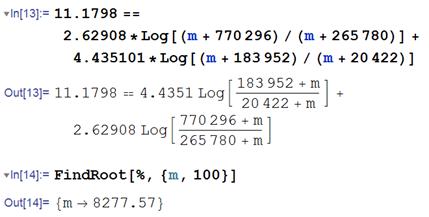
so
the solution is 8300kg a very small mass compared with that of the
launch vehicle, but you could pack in a large number of people you would like
to launch into outer space nonetheless (the entire faculty of the division of
engineering, if you wish).
4.2.7 Analyzing collisions between particles: the restitution coefficient
The momentum conservation equations are particularly helpful if you want to analyze collisions between two or more objects. If the impact occurs over a very short time, the impulse exerted by the contact forces acting at the point of collision is huge compared with the impulse exerted by any other forces. If we consider the two colliding particles as a system, the external impulse exerted on the system can be taken to be zero, and so the total momentum of the system is conserved.
The
momentum conservation equation can be used to relate the velocities of the
particles before collision to those after collision. These relations are not enough to be able to
determine the velocities completely, however to do this, we also need to be able to
quantify the energy lost (or more accurately, dissipated as heat) during the
collision.
In
practice we don’t directly specify the energy loss during a collision instead, the relative velocities are related
by a property of the impact called the coefficient
of restitution.
Restitution coefficient for straight line motion
Suppose that two colliding particles A and B move in a straight line parallel to a unit vector i. Let
denote the velocities of A and B just before
the collision
denote the velocities of A and B just after
the collision.
The velocities before and after impact are related by
where e is the restitution coefficient. The negative sign is needed because the particles approach one another before impact, and separate afterwards.
Restitution coefficient for 3D frictionless collisions
For a more general contact, we define
to denote velocities of the particles before
collision
to denote velocities of the particles after
collision
In addition, we let n be a unit vector normal to the common tangent plane at the point of contact (if the two colliding particles are spheres or disks the vector is parallel to the line joining their centers).
The velocities before and after impact are related by two vector equations:
To interpret these equations, note that
1. The first equation states that the component of relative velocity normal to the contact plane is reduced by a factor e (just as for 1D contacts)
2. The second equation states that the component of relative velocity tangent to the contact plane is unchanged (this is because the contact is frictionless, and so the reaction forces acting on the particles during the collision exert no impulse is exerted in a direction tangent to the contact plane).
The
two equations can be combined into a single vector equation relating velocities
before and after impact this form is more compact, and often more
useful, but more difficult to visualize physically
It is possible to account for friction at the contact, but friction will always make the colliding particles rotate, so they cannot be idealized as particles.
Values of restitution coefficient
The
restitution coefficient almost always lies in the range . It can only be less than zero if one object
can penetrate and pass through the other (e.g. a bullet); and can only be
greater than 1 if the collision generates energy somehow (e.g. releasing a
preloaded spring, or causing an explosion).
If e=0, the two colliding objects stick together; if e=1 the collision is perfectly elastic, with no energy loss.
The restitution coefficient is strongly sensitive to the material properties of the two colliding objects, and also varies weakly with their geometry and the velocity of impact. The two latter effects are usually ignored.
Collision between a particle and a fixed rigid surface. The collision formulas can be applied to impact between a rigid fixed surface by taking the surface to be particle B, and noting that the velocity of particle B is then zero both before and after impact.
For straight line motion,
For
collision with an angled wall ,
where
n is a unit vector perpendicular to the wall.
4.2.8 Examples of collision problems
Example 1 Suppose that a moving car hits a stationary (parked) vehicle from behind. Derive a formula that will enable an accident investigator to determine the velocity of the moving car from the length of the skid marks left on the road.
Assumptions:
1. We will assume both cars move in a straight line
2.
The moving and
stationary cars will be assumed to have masses ,
respectively
3. We will assume the cars stick together after the collision (i.e. the restitution coefficient is zero)
4. We will assume that only the parked car has brakes applied after the collision
This calculation takes two steps: first, we will use work-energy to relate the distance slid by the cars after impact to their velocity just after the impact occurs. Then, we will use momentum and the restitution formula to work out the velocity of the moving car just before impact.
Calculation:
Let V denote the velocity of the moving car just before impact; let denote the velocity of the two (connected)
cars just after impact, and let d denote
the distance slid.
1. The figure shows a free body diagram for each of the
two cars during sliding after the collision.
2.
The vertical
component of the equations of motion give ;
.
3. The parked car has locked wheels and skids over the
road; the friction law gives the tangential forces at the contacts as
4. We can calculate the velocity of the cars just after
impact using the work-kinetic energy relation during skidding. For this purpose, we consider the two
connected cars as a single particle. The
work done on the particle by the friction forces is . The work done is equal to the change in
kinetic energy of the particle, so
5. Finally, we can use momentum conservation to calculate
the velocity just before impact. The
momentum after impact is ,
while before impact
. Equating the two gives
Example 2: Two frictionless spheres with radius R have initial velocity . At some instant of time, the two particles
collide. At the point of collision, the centers
of the spheres have position vectors
. The restitution coefficient for the contact
is denoted by e. Find a formula for
the velocities of the spheres after impact.
Hence, deduce an expression for the change in kinetic energy during the
impact.
This is a
straightforward vector algebra exercise.
We have two unknown velocity vectors: ,
and two vector equations
momentum conservation, and the restitution
coefficient formula.
Calculation
1. Note that a unit vector normal to the tangent plane
can be calculated from the position vectors of the centers at the impact as . It doesn’t matter whether you choose to take n to point from A to B or the other way
around
the formula will work either way.
2. Momentum conservation requires that
3. The restitution coefficient formula gives
4. We can solve (2) and (3) for by multiplying (3) by
and adding the equations, which gives
5. Similarly, we can solve for by multiplying (3) by
and subtracting (3) from (2), with the result
6. The change in kinetic energy during the collision can be calculated as
7.
Substituting the
results of (4) and (5) for and
and simplifying the result gives
Note that the energy change is zero if e=1 (perfectly elastic collisions) and is always negative for e<1 (i.e. the kinetic energy after collision is less than that before collision).
 Example 3: This
is just a boring example to help illustrate the practical application of the
vector formulas in the preceding example.
In the figure shown, disk A
has a vertical velocity V at time t=0, while disk B is stationary. The two disks both have radius R, have the same mass, and the
restitution coefficient between them is e.
Gravity can be neglected. Calculate the velocity vector of each disk after
collision.
Example 3: This
is just a boring example to help illustrate the practical application of the
vector formulas in the preceding example.
In the figure shown, disk A
has a vertical velocity V at time t=0, while disk B is stationary. The two disks both have radius R, have the same mass, and the
restitution coefficient between them is e.
Gravity can be neglected. Calculate the velocity vector of each disk after
collision.
Calculation
1. Before impact, the velocity vectors are
2. A unit vector parallel to the line joining the two
centers is (to see this, apply Pythagoras theorem to the
triangle shown in the figure).
3. The velocities after impact are
Substituting the vectors gives
 Example 4: How
to play pool (or snooker, billiards, or your own favorite bar game involving
balls, a stick, and a table…). The
figure shows a typical problem faced by a pool player
Example 4: How
to play pool (or snooker, billiards, or your own favorite bar game involving
balls, a stick, and a table…). The
figure shows a typical problem faced by a pool player where should the queue ball hit the eight ball
to send it into the pocket?
This
is easily solved the eight ball is stationary before impact,
and after impact has a velocity
Notice that the velocity is parallel to the unit vector n. This vector is parallel to a line connecting the centers of the two balls at the instant of impact. So the correct thing to do is to visualize an imaginary ball just touching the eight ball, in line with the pocket, and aim the queue ball at the imaginary ball. Easy!
 The real
secret to being a successful pool player is not potting the balls
The real
secret to being a successful pool player is not potting the balls that part is easy. It is controlling where the queue ball goes
after impact. You may have seen experts
make a queue ball reverse its direction after an impact (appearing to bounce
off the stationary ball); or make the queue ball follow the struck ball after
the impact. According to the simple
equations developed here, this is impossible
but a pool table is more complicated, because
the balls rotate, and are in contact with a table. By giving the queue ball spin, an expert player can move the queue ball around at will. To make the ball rebound, it must be struck
low down (below the ‘center of percussion’) to give it a reverse spin; to make
it follow the struck ball, it should be struck high up, to make it roll towards
the ball to be potted. Giving the ball
a sideways spin can make it rebound in a controllable direction laterally as
well. And it is even possible to make a
queue ball travel in a curved path
with the right spin.
Never let it be said that you don’t learn useful skills in engineering classes!
 Example 5: In
this problem we set up a simple MATLAB program that analyzes motion with
impacts. The problem to be solved in
illustrated in the figure. A square box
contains a number of rigid, frictionless circular disks. The disks all have the same mass. At time t=0
the disks are given some random distribution of velocities. The goal of the program is to compute and
animate the subsequent motion of the disks, accounting for all collisions.
Example 5: In
this problem we set up a simple MATLAB program that analyzes motion with
impacts. The problem to be solved in
illustrated in the figure. A square box
contains a number of rigid, frictionless circular disks. The disks all have the same mass. At time t=0
the disks are given some random distribution of velocities. The goal of the program is to compute and
animate the subsequent motion of the disks, accounting for all collisions.
To do this, we need to:
1. Derive the equations of motion for each disk and integrate them;
2. Detect collisions between particles and the wall, and change the particle velocity to account for the collision;
3. Detect collisions between two particles, and change the velocities of both colliding particles to account for the collision.
We will model the system by
calculating the (x,y) coordinates of
each disk. In the following, we will use
to denote the position and velocity of the ith disk.
Equations of motion : No forces act on the disks except during the collisions. Therefore, between collisions, the equations of motion for the ith disk is
As always, we turn this into MATLAB form by writing
Collisions with the walls: The collisions occur at the instants when the distance of a disk to the wall is equal to the radius of the disk. Therefore
1.
Collision with
the wall at x=L occurs when
2.
Collision with the wall at x=-L
3.
Collision with the roof at y=L occurs when
4.
Collision with the floor at y=-L occurs when
A collision can be detected by detecting the point when
crosses zero from above.
When a collision occurs, the velocities must be corrected as follows to account for the collision:
1.
Collision with
the walls at
2.
Collision with
the walls at
Collisions between particles The collisions occur at the instants when the distance between the centers of any two disks is equal to the diameter of the disk.
When a collision occurs between the ith and jth particles, their velocities must be corrected as follows to account for the collision:
To see this, note that is a unit vector joining the two centers; and
let
denote the velocities of the two particles,
and substitute into the general equations in Example 4.
Here
is a MATLAB script that implements these calculations. It will produce the
animation shown in the picture. You can
make various modifications to solve similar problems. The only new feature of this code that has
not been discussed before is the ODE solver it turns out that the standard solver ode45 is
not accurate enough for this problem and misses some collisions. The more accurate solver ode113 is used
instead.
function disk_collisions
% Function to compute and animate motion of colliding disks
% in a box
n_disks = 3;
disk_radius = 1;
box_size = 10.0;
restitution_wall = 1;
restitution_disk = 1;
% These variables are defined in the outer function so they are available
% in all functions
disk_wall_index = 1; %specifies the disk that is closest to a wall
colliding_pair(1) = 1; %specifies first disk in pair of closest disks
colliding_pair(2) = 1; %specifies second disk in pair of closest disks
tstart = 0;
tstop = 60;
count = 0;
y0 = [1.,1.,0.,0.,-1.,-1.1,1.,1.,-3.,3.,-0.25,0.25];
while(tstart<tstop)
Abstol = 10^(-05)*ones(4*n_disks,1);
options = odeset('RelTol',0.0000001,'AbsTol',Abstol,'Events',@detect_collision);
[t,y,tevent,yevent,ievent] = ode113(@eom,[tstart,tstop],y0,options);
if (~isempty(tevent))
y0 = collide(tevent,yevent,ievent);
end
tstart = t(length(t));
for i=1:length(t)
% The disks are a single point on an x-y plot
hold off
plot(y(i,1),y(i,2),'ro','MarkerSize',52,'MarkerFaceColor','r');
hold on
for n = 2:n_disks
plot(y(i,4*(n-1)+1),y(i,
4*(n-1)+2),'ro','MarkerSize',52,'MarkerFaceColor','r');
end
axis([-5,5,-5,5]);
axis square
pause(0.025) % This just slows down the animation a bit
end
end
function dydt = eom(t,y)
% Equations of motion for the disks
% y contains [x,y,vx,vy,…] for each disk
for n=1:n_disks
i = 4*(n-1)+1;
dydt(i) = y(i+2);
dydt(i+1) = y(i+3);
dydt(i+2) = 0;
dydt(i+3) = 0.;
end
dydt = transpose(dydt);
end
function [eventvalue,stopthecalc,eventdirection] = detect_collision(t,y)
% Function to detect a collision of a disk with a wall or another disk
%
% Find the shortest distance between a disk and a wall
dmin = box_size;
for n=1:n_disks
i = 4*(n-1)+1;
d1 = box_size/2-(y(i)+disk_radius);
d2 = (y(i)-disk_radius)+box_size/2;
d3 = box_size/2-(y(i+1)+disk_radius);
d4 = (y(i+1)-disk_radius)+box_size/2;
[d,min_wall] = min([d1,d2,d3,d4]);
if (d<dmin)
dmin = d;
disk_wall_index = n;
end
end
% First event is collision of disk with a wall
eventvalue(1) = dmin;
stopthecalc(1) = 1;
eventdirection(1)=-1;
dmin = 10*box_size;
% Find the min dist between any pair of disks
if (n_disks>1)
for n=1:n_disks-1
i = 4*(n-1)+1;
for m = n+1:n_disks
j = 4*(m-1)+1;
d = sqrt( (y(j)-y(i))^2 + (y(j+1)-y(i+1))^2)-2*disk_radius;
if (d<dmin)
dmin = d;
colliding_pair(1)=n;
colliding_pair(2)=m;
end
end
end
% Second event is collision of two disks
eventvalue(2) = dmin;
stopthecalc(2) = 1;
eventdirection(2)=-1;
end
end
function y0 = collide(t,y,ievent)
% Function to change velocity of disks when a collision occurs
y0 = y;
if (ievent==1) %collision with a wall
i = 4*(disk_wall_index-1)+1;
d1 = box_size/2-(y(i)+disk_radius);
d2 = (y(i)-disk_radius)+box_size/2;
d3 = box_size/2-(y(i+1)+disk_radius);
d4 = (y(i+1)-disk_radius)+box_size/2;
if (d1<0.0001 || d2<0.0001) %collision with left or right wall
y0(i+2) = -restitution_wall*y0(i+2);
end
if (d3<0.0001 || d4<0.0001) % collision with top or bottom wall
y0(i+3) = -restitution_wall*y0(i+3);
end
else
i = 4*(colliding_pair(1)-1)+1;
j = 4*(colliding_pair(2)-1)+1;
normal(1) = (y(j)-y(i))/(2*disk_radius);
normal(2)= (y(j+1)-y(i+1))/(2*disk_radius);
vn = (y(j+2)-y(i+2))*normal(1) + (y(j+3)-y(i+3))*normal(2);
y0(i+2) = y0(i+2) + (1+restitution_disk)*vn*normal(1)/2;
y0(i+3) = y0(i+3) + (1+restitution_disk)*vn*normal(2)/2;
y0(j+2) = y0(j+2) - (1+restitution_disk)*vn*normal(1)/2;
y0(j+3) = y0(j+3) - (1+restitution_disk)*vn*normal(2)/2;
end
end
end