
Chapter 4
Conservation laws for systems of particles
In this chapter, we shall introduce (but not in this order) the following general concepts:
- The linear impulse of a force
- The angular impulse of a force
- The power transmitted by a force
- The work done by a force
- The potential energy of a force.
- The linear momentum of a particle (or system of particles)
- The angular momentum of a particle, or system of particles.
- The kinetic energy of a particle, or system of particles
- The linear impulse momentum relations for a particle, and conservation of linear momentum
- The principle of conservation of angular momentum for a particle
- The principle of conservation of energy for a particle or system of particles.
We will also illustrate how these concepts can be used in engineering calculations. As you will see, to applying these principles to engineering calculations you will need two things: (i) a thorough understanding of the principles themselves; and (ii) Physical insight into how engineering systems behave, so you can see how to apply the theory to practice. The first is easy. The second is hard, and people who can do this best make the best engineers.
4.1 Work, Power, Potential Energy and Kinetic Energy relations
The
concepts of work, power and energy are among the most powerful ideas in the
physical sciences. Their most important
application is in the field of thermodynamics,
which describes the exchange of energy between interacting systems. In addition, concepts of energy carry over to
relativistic systems and quantum mechanics, where the classical versions of
In this section, we develop the basic definitions of mechanical work and energy, and show how they can be used to analyze motion of dynamical systems. Future courses will expand on these concepts further.
4.1.1 Definition of the power and work done by a force
Suppose that a force F acts on a particle that moves with speed v.
By definition:
![]() The Power
developed by the force, (or the rate of
work done by the force) is
The Power
developed by the force, (or the rate of
work done by the force) is . If both force and velocity are expressed in
Cartesian components, then
Work
has units of Nm/s, or `
![]() The work done by the force during a time interval
The work done by the force during a time interval is
The work done by the force can also be calculated by integrating the force vector along the path traveled by the force, as
where
are the initial and final positions of the
force.
Work has units of Nm in SI units, or `Joules’
A moving force can do work on a particle, or on any moving object. For example, if a force acts to stretch a spring, it is said to do work on the spring.
4.1.2 Definition of the power and work done by a concentrated moment, couple or torque.
 ‘Concentrated moment, ‘Couple’ and `Torque’ are
different names for a ‘generalized force’ that causes rotational motion without
causing translational motion. These
concepts are not often used to analyze motion of particles, where rotational
motion is ignored
‘Concentrated moment, ‘Couple’ and `Torque’ are
different names for a ‘generalized force’ that causes rotational motion without
causing translational motion. These
concepts are not often used to analyze motion of particles, where rotational
motion is ignored the only application might be to analyze
rotational motion of a massless frame connected to one or more particles. For completeness, however, the power-work
relations for moments are listed in this section and applied to some simple
problems. To do this, we need briefly to
discuss how rotational motion is
described. This topic will be developed
further in Chapter 6, where we discuss motion of rigid bodies.
Definition
of an angular velocity vector Visualize
a spinning object, like the cube shown in the figure. The box rotates about an axis in the example, the axis is the line
connecting two cube diagonals. In
addition, the object turns through some number of revolutions every
minute. We would specify the angular
velocity of the shaft as a vector
,
with the following properties:
- The direction of the vector is parallel to the axis of the shaft (the axis of rotation). This direction would be specified by a unit vector n parallel to the shaft
- There are, of course, two possible directions for n. By convention, we always choose a direction such that, when viewed in a direction parallel to n (so the vector points away from you) the shaft appears to rotate clockwise. Or conversely, if n points towards you, the shaft appears to rotate counterclockwise. (This is the `right hand screw convention’)
|
|
|
|
Viewed along n |
Viewed in direction opposite to n |


- The magnitude of the
vector is the angular speed of the object, in radians per second. If you know the revs per minute n turned by the shaft, the number of radians per sec follows as. The magnitude of the angular velocity is often denoted by
The
angular velocity vector is then .
Since
angular velocity is a vector, it has components in a fixed Cartesian basis.
Rate
of work done by a torque or moment: If
a moment acts
on an object that rotates with angular velocity
,
the rate of work done on the object by M
is
4.1.3 Simple examples of power and work calculations
Example 1: An aircraft with mass 45000 kg flying at 200 knots (102m/s) climbs at 1000ft/min. Calculate the rate of work done on the aircraft by gravity.
The gravitational force is ,
and the velocity vector of the aircraft is
. The rate of work done on the aircraft is
therefore
Substituting numbers gives
 Example 2:
Calculate a formula for the work required to
stretch a spring with stiffness k and
unstretched length
Example 2:
Calculate a formula for the work required to
stretch a spring with stiffness k and
unstretched length from length
to length
.
The
figure shows a spring that held fixed at A
and is stretched in the horizontal direction by a force acting at B. At some instant the spring has length
. The spring force law states that the force
acting on the spring at B is related to the length of the spring x by
The position vector of the
force is ,
and therefore the work done is
 Example 3:
Calculate the work done by gravity on a
satellite that is launched from the surface of the earth to an altitude of
250km (a typical low earth orbit).
Example 3:
Calculate the work done by gravity on a
satellite that is launched from the surface of the earth to an altitude of
250km (a typical low earth orbit).
Assumptions
- The earth’s radius is 6378.145km
- The mass of a typical satellite is 4135kg - see , e.g. http://www.astronautix.com/craft/hs601.htm
- The Gravitational parameter (G= gravitational constant; M=mass of earth)
- We will assume that the satellite is launched along a straight line path parallel to the i direction, starting the earths surface and extending to the altitude of the orbit. It turns out that the work done is independent of the path, but this is not obvious without more elaborate and sophisticated calculations.
Calculation:
- The gravitational force on the satellite is
- The work done follows as
- Substituting numbers gives J (be careful with unitsif you work with kilometers the work done is in N-km instead of SI units Nm)
 Example 4: A Ferrari Testarossa skids to a stop over a distance
of 250ft. Calculate the total work done
on the car by the friction forces acting on its wheels.
Example 4: A Ferrari Testarossa skids to a stop over a distance
of 250ft. Calculate the total work done
on the car by the friction forces acting on its wheels.
Assumptions:
- A Ferrari Testarossa has mass 1506kg (see http://www.ultimatecarpage.com/car/1889/Ferrari-Testarossa.html)
- The coefficient of friction between wheels and road is of order 0.8
- We assume the brakes are locked so all wheels skid, and air resistance is neglected
Calculation The figure shows a free body diagram. The equation of motion for the car is
- The vertical component of the equation of motion
yields
- The friction law shows that
- The position vectors of the car’s front and rear
wheels are . The work done follows as. We suppose that the rear wheel starts at some pointwhen the brakes are applied and skids a total distance d.
- The work done follows as . Substituting numbers gives.
 Example 5: The figure shows a box that is pushed up a slope by a
force P. The box moves with speed v. Find a formula for the rate of work done by each of the forces
acting on the box.
Example 5: The figure shows a box that is pushed up a slope by a
force P. The box moves with speed v. Find a formula for the rate of work done by each of the forces
acting on the box.
The figure shows a free body diagram. The force vectors are
1.
Applied force
2.
Friction
3.
Normal reaction
4.
Weight
The velocity vector is
Evaluating the dot products for each
formula, and recalling that
gives
1.
Applied force
2.
Friction
3.
Normal reaction
4.
Weight
|
Force N |
Draw (cm) |
|
0 |
0 |
|
40 |
10 |
|
90 |
20 |
|
140 |
30 |
|
180 |
40 |
|
220 |
50 |
|
270 |
60 |
Example 6: The table lists the experimentally measured force-v-draw data for a long-bow. Calculate the total work done to draw the bow.
In this case we don’t have a function that specifies the force as a function of position; instead, we have a table of numerical values. We have to approximate the integral
 numerically. To
understand how to do this, remember that integrating a function can be
visualized as computing the area under a curve of the function, as illustrated
in the figure.
numerically. To
understand how to do this, remember that integrating a function can be
visualized as computing the area under a curve of the function, as illustrated
in the figure.
We can estimate the integral by dividing the area into a series of trapezoids, as shown. Recall that the area of a trapezoid is (base x average height), so the total area of the function is
You could easily do this
calculation by hand but for lazy people like me MATLAB has a
convenient function called `trapz’ that does this calculation
automatically. Here’s how to use it
>> draw = [0,10,20,30,40,50,60]*0.01;
>> force = [0,40,90,140,180,220,270];
>> trapz(draw,force)
ans =
80.5000
>>
So the solution is 80.5J
 4.1.4 Definition
of the potential energy of a conservative force
4.1.4 Definition
of the potential energy of a conservative force
Preamble: Textbooks nearly always define the `potential energy
of a force.’ Strictly speaking, we
cannot define a potential energy of a single force instead, we need to define the potential
energy of a pair of forces. A force
can’t exist by itself
there must always be an equal and opposite
reaction force acting on a second body.
In all of the discussion to be presented in this section, we
implicitly assume that the reaction force is acting on a second body, which is
fixed at the origin. This
simplifies calculations, and makes the discussion presented here look like
those given in textbooks, but you should remember that the potential energy of
a force pair is always a function of the relative positions of the two forces.
With that proviso, consider a
force F acting on a particle at some
position r in space. Recall that the
work done by a force that moves from position vector to position vector
is
In general, the work done by
the force depends on the path between to
. For some special forces, however, the work
done is independent of the path. Such
forces are said to be conservative.
For a force to be conservative:
![]() The force must be a function only of its
position
The force must be a function only of its
position i.e. it can’t depend on the velocity of the
force, for example.
![]() The force vector must satisfy
The force vector must satisfy
Examples of conservative forces include gravity, electrostatic forces, and the forces exerted by a spring. Examples of non-conservative (or should that be liberal?) forces include friction, air resistance, and aerodynamic lift forces.
The
potential
energy of a conservative force is defined as the negative of the work
done by the force in moving from some arbitrary initial position to a new position
,
i.e.
The
constant is arbitrary, and the negative sign is introduced by convention (it
makes sure that systems try to minimize their potential energy). If there is a point where the force is zero,
it is usual to put at this point, and take the constant to be
zero.
Note that
- The potential energy is a scalar valued function
- The potential energy
is a function only of the position of the force. If we choose to describe position in
terms of Cartesian components , then.
- The relationship between potential energy and force can also be expressed in differential form (which is often more useful for actual calculations) as
If we choose to work with Cartesian components, then
Occasionally,
you might have to calculate a potential energy function by integrating forces for example, if you are interested in running a molecular
dynamic simulation of a collection of atoms in a material, you will need to describe
the interatomic forces in some convenient way.
The interatomic forces can be estimated by doing quantum-mechanical
calculations, and the results can be approximated by a suitable potential
energy function. Here are a few examples
showing how you can integrate forces to calculate potential energy
 Example 1: Potential energy of forces exerted by a
spring. A free body diagram showing the forces
exerted by a spring connecting two objects is shown in the figure.
Example 1: Potential energy of forces exerted by a
spring. A free body diagram showing the forces
exerted by a spring connecting two objects is shown in the figure.
- The force exerted by a spring is
- The position vector of the force is
- The potential energy follows as
where we have taken the constant to be zero.
Example 2: Potential energy of electrostatic forces exerted by charged particles.
The figure shows two charged particles a distance x apart. To calculate the potential energy of the force acting on particle 2, we place particle 1 at the origin, and note that the force acting on particle 2 is
where
and
are the charges on the two particles, and
is a fundamental physical constant known as
the Permittivity of the medium
surrounding the particles. Since the
force is zero when the particles are infinitely far apart, we take
at infinity.
The potential energy follows as
Table of potential energy relations
In practice, however, we rarely need to do the integrals to calculate the potential energy of a force, because there are very few different kinds of force. For most engineering calculations the potential energy formulas listed in the table below are sufficient.
|
Type of force |
Force vector |
Potential energy |
|
|
Gravity acting on a particle near earths surface |
|
|
|
|
Gravitational force exerted on mass m by mass M at the origin |
|
|
|
|
Force exerted by a spring with stiffness k and unstretched length |
|
|
|
|
Force acting between two charged particles |
|
|
|
|
Force exerted by one molecule of a noble gas (e.g. He, Ar, etc) on another (Lennard Jones potential). a is the equilibrium spacing between molecules, and E is the energy of the bond. |
|
|
|
4.1.5 Potential energy of concentrated moments exerted by a torsional spring

A potential energy cannot usually be defined for concentrated moments, because rotational motion is itself path dependent (the orientation of an object that is given two successive rotations depends on the order in which the rotations are applied). A potential energy can, however, be defined for the moments exerted by a torsional spring.
A
solid rod is a good example of a torsional spring. You could take hold of the
ends of the rod and twist them, causing one end to rotate relative to the
other. To do this, you would apply a moment or a couple to each end of the rod, with direction parallel to the axis
of the rod. The angle of twist
increases with the moment. Various
torsion spring designs used in practice are shown in the picture the image is from
http://www.mollificio.lombardo.molle.com/springs/torsion_springs.html
More generally, a torsional spring resists rotation, by exerting equal and opposite moments on objects connected to its ends. For a linear spring the moment is proportional to the angle of rotation applied to the spring.
 The figure shows a formal free body diagram for two
objects connected by a torsional spring.
If object A is held fixed, and
object B is rotated through an angle
The figure shows a formal free body diagram for two
objects connected by a torsional spring.
If object A is held fixed, and
object B is rotated through an angle about an axis parallel to a unit vector n, then the spring exerts a moment
on object B where is the torsional
stiffness of the spring. Torsional
stiffness has units of Nm/radian.
The
potential energy of the moments exerted by the spring can be determined by
computing the work done to twist the spring through an angle .
- The work done by a
moment M due to twisting
through a very small angle about an axis parallel to a vector n is
- The potential energy is the negative of the total work done by M, i.e.
 4.1.6
Definition of the Kinetic Energy of a particle
4.1.6
Definition of the Kinetic Energy of a particle
Consider a particle with mass
m which moves with velocity . By definition, its kinetic energy is
|
|
|
4.1.7 Power-Work-kinetic energy relations for a single particle
Consider a particle with mass m that moves under the action of a force F. Suppose that
- At some time the particle has some initial position, velocityand kinetic energy
- At some later time the particle has a new position r, velocityand kinetic energy.
- Let denote the rate of work done by the force
- Let be the total work done by the force
The Power-kinetic energy relation for the particle states that the rate of work done by F is equal to the rate of change of kinetic energy of the particle, i.e.
|
|
|
This
is just another way of writing
|
|
|
To see the last step, do the
derivative using the Chain rule and note that .
The Work-kinetic energy relation for a particle says that the total work done by the force F on the particle is equal to the change in the kinetic energy of the particle.
This follows by integrating the power-kinetic energy relation with respect to time.
4.1.8 Examples of simple calculations using work-power-kinetic energy relations
There are two main applications of the work-power-kinetic energy relations. You can use them to calculate the distance over which a force must act in order to produce a given change in velocity. You can also use them to estimate the energy required to make a particle move in a particular way, or the amount of energy that can be extracted from a collection of moving particles (e.g. using a wind turbine)
Example 1: Estimate the minimum distance required for a 14 wheeler that travels at the RI speed-limit to brake to a standstill. Is the distance to stop any different for a Toyota Echo?
This
problem can be solved by noting that, since we know the initial and final speed
of the vehicle, we can calculate the change in kinetic energy as the vehicle
stops. The change in kinetic energy must
equal the work done by the forces acting on the vehicle which depends on the distance slid. Here are the details of the calculation.
 Assumptions:
- We assume that all the wheels are locked and skid over the ground (this will stop the vehicle in the shortest possible distance)
- The contacts are
assumed to have friction coefficient
- The vehicle is idealized as a particle.
- Air resistance will be neglected.
Calculation:
- The figure shows a free body diagram.
- The equation of motion for the vehicle is
The vertical component of the equation shows that .
- The friction force
follows as
- If the vehicle skids for a distance d, the total work done by the forces acting on the vehicle is
- The work-energy relation states that the total
work done on the particle is equal to its change in kinetic energy. When the brakes are applied the vehicle
is traveling at the speed limit, with speed V; at the end of the skid its speed is zero. The change in kinetic energy is
therefore . The work-energy relation shows that
Substituting numbers gives
This
simple calculation suggests that the braking distance for a vehicle depends
only on its speed and the friction coefficient between wheels and tires. This is unlikely to vary much from one
vehicle to another. In practice there
may be more variation between vehicles than this estimate suggests, partly because
factors like air resistance and aerodynamic lift forces will influence the results,
and also because vehicles usually don’t skid during an emergency stop (if they
do, the driver loses control) the nature of the braking system therefore
also may change the prediction.
Example 3: Compare the power consumption of a Ford Excursion to that of a Chevy Cobalt during stop-start driving in a traffic jam.
During stop-start driving, the vehicle must be repeatedly accelerated to some (low) velocity; and then braked to a stop. Power is expended to accelerate the vehicle; this power is dissipated as heat in the brakes during braking. To calculate the energy consumption, we must estimate the energy required to accelerate the vehicle to its maximum speed, and estimate the frequency of this event.
Calculation/Assumptions:
- We assume that the speed in a traffic jam is low enough that air resistance can be neglected.
- The energy to
accelerate to speed V is .
- We assume that the
vehicle accelerates and brakes with constant acceleration if so, its average speed is V/2.
- If the vehicle travels a distance d between stops, the time between two stops is 2d/V.
- The average power is
therefore .
- Taking V=15mph (7m/s) and d=200ft (61m) are reasonable values
the power is therefore 0.03m, with m in kg. A Ford Excursion weighs 9200 lb (4170 kg), requiring 125 Watts (about that of a light bulb) to keep moving. A Chevy Cobalt weighs 2681lb (1216kg) and requires only 36 Wattsa very substantial energy saving.
Reducing
vehicle weight is the most effective way of improving fuel efficiency during
slow driving, and also reduces manufacturing costs and material requirements. Another, more costly, approach is to use a
system that can recover the energy during braking this is the main reason that hybrid vehicles
like the Prius have better fuel economy than conventional vehicles.
 Example 4: Estimate the power that can be generated by a wind
turbine.
Example 4: Estimate the power that can be generated by a wind
turbine.
The
figure shows a wind turbine. The turbine
blades deflect the air flowing past them: this changes the air speed and so
exerts a force on the blades. If the
blades move, the force exerted by the air on the blades does work this work is the power generated by the
turbine. The rate of work done by the
air on the blades must equal the change in kinetic energy of the air as it
flows past the blades. Consequently, we
can estimate the power generated by the turbine by calculating the change in
kinetic energy of the air flowing through it.
To do this properly needs a very sophisticated analysis of the air flow around the turbine. However, we can get a rather crude estimate of the power by assuming that the turbine is able to extract all the energy from the air that flows through the circular area swept by the blades.
Calculation: Let V
denote the wind speed, and let denote the density of the air.
1. In a time t, a cylindrical region of air with radius R and height Vt passes through the fan.
2. The cylindrical region has mass
3. The kinetic energy of the cylindrical region of air is
4. The rate of flow of kinetic energy through the fan is
therefore
5. If all this energy could be used to do work on the fan
blades the power generated would be
Representative
numbers are (i) Air density 1.2 ;
(ii) air speed 25mph (11 m/sec); (iii) Radius 30m
This gives 1.8MW. For comparison, a nuclear power plant generates about 500-1000 MW.
A more sophisticated calculation (which will be covered in EN810) shows that in practice the maximum possible amount of energy that can be extracted from the air is about 60% of this estimate. On average, a typical household uses about a kW of energy; so a single turbine could provide enough power for about 5-10 houses.
4.1.9 Energy relations for a conservative system of particles.
 The figure shows a `system of particles’
 this is just a collection of objects that we
might be interested in, which can be idealized as particles. Each particle in the system can
experience forces applied by:
![]() Other particles in the system (e.g.
due to gravity, electric charges on the particles, or because the particles are
physically connected through springs, or because the particles collide). We call these internal forces acting in
the system. We will denote the internal
force exerted by the ith particle on
the jth particle by
Other particles in the system (e.g.
due to gravity, electric charges on the particles, or because the particles are
physically connected through springs, or because the particles collide). We call these internal forces acting in
the system. We will denote the internal
force exerted by the ith particle on
the jth particle by . Note that, because every action has an equal
and opposite reaction, the force exerted on the jth particle by the ith
particle must be equal and opposite, to
,
i.e.
.
![]() Forces exerted on the particles by the outside
world (e.g. by externally applied gravitational or electromagnetic
fields, or because the particles are connected to the outside world through
mechanical linkages or springs). We call
these external forces acting on the system, and we will denote the external
force on the i th particle by
Forces exerted on the particles by the outside
world (e.g. by externally applied gravitational or electromagnetic
fields, or because the particles are connected to the outside world through
mechanical linkages or springs). We call
these external forces acting on the system, and we will denote the external
force on the i th particle by
We
define the total external work done on
the system during a time interval as the sum of the work done by the external
forces.
The total work done can also include a contribution from external moments acting on the system.
The system of particles is conservative if all the internal forces in the system are conservative. This means that the particles must interact through conservative forces such as gravity, springs, electrostatic forces, and so on. The particles can also be connected by rigid links, or touch one another, but contacts between particles must be frictionless.
If this is the case, we can define the total potential energy of the system as the sum of potential energies of all the internal forces.
We
also define the total kinetic energy of the system as the sum of kinetic energies
of all the particles.
The work-energy relation for the system of particles can then be stated as follows. Suppose that
- At some time the system has and kinetic energy
- At some later time the system has kinetic energy.
- Let denote the potential energy of the force at time
- Let denote the potential energy of the force at time
- Let denote the total work done on the system between
Work Energy Relation: This law states that the external work done on the system is equal to the change in total kinetic and potential energy of the system.
We won’t attempt to prove
this result - the proof is conceptually
very straightforward: it simply involves summing the work-energy relation for
all the particles in the system; and we’ve already seen that the work-energy
relations are simply a different way of writing
Energy conservation law For the special case where no external forces act on the system, the total energy of the system is constant
It
is worth making one final remark before we turn to applications of these
law. We often invoke the principle of
conservation of energy when analyzing the motion of an object that is subjected
to the earth’s gravitational field. For
example, the first problem we solve in the next section involves the motion of
a projectile launched from the earth’s surface.
We usually glibly say that `the sum of the potential and kinetic
energies of the particle are constant’ and if you’ve done physics courses you’ve
probably used this kind of thinking. It
is not really correct, although it leads to a more or less correct solution.
Properly, we should consider the earth and the projectile together as a conservative system. This means we must include the kinetic energy of the earth in the calculation, which changes by a small, but finite, amount due to gravitational interaction with the projectile. Fortunately, the principle of conservation of linear momentum (to be covered later) can be used to show that the change in kinetic energy of the earth is negligibly small compared to that of the particle.
4.1.10 Examples of calculations using kinetic and potential energy in conservative systems
The kinetic-potential energy relations can be used to quickly calculate relationships between the velocity and position of an object. Several examples are provided below.
Example 1: (Boring FE exam question) A projectile with mass m is launched from the ground with velocity at angle
. Calculate an expression for the maximum
height reached by the projectile.
If air resistance can be neglected, we can regard the earth and the projectile together as a conservative system. We neglect the change in the earth’s kinetic energy. In addition, since the gravitational force acting on the particle is vertical, the particle’s horizontal component of velocity must be constant.
Calculation:
- Just after launch, the velocity of the particle
is
- The kinetic energy of the particle just after
launch is . Its potential energy is zero.
- At the peak of the trajectory the vertical
velocity is zero. Since the horizontal velocity remains constant, the
velocity vector at the peak of the trajectory is . The kinetic energy at this point is therefore
- Energy is conserved, so
 Example 2: You are asked to design the packaging for a sensitive
instrument. The packaging will be made
from an elastic foam, which behaves like a spring. The specifications restrict
the maximum acceleration of the instrument to 15g. Estimate the thickness of the packaging that
you must use.
Example 2: You are asked to design the packaging for a sensitive
instrument. The packaging will be made
from an elastic foam, which behaves like a spring. The specifications restrict
the maximum acceleration of the instrument to 15g. Estimate the thickness of the packaging that
you must use.
This problem can be solved by noting that (i) the max acceleration occurs when the packaging (spring) is fully compressed and so exerts the maximum force on the instrument; (ii) The velocity of the instrument must be zero at this instant, (because the height is a minimum, and the velocity is the derivative of the height); and (iii) The system is conservative, and has zero kinetic energy when the package is dropped, and zero kinetic energy when the spring is fully compressed.
 Assumptions:
- The package is dropped from a height of 1.5m
- The effects of air resistance during the fall are neglected
- The foam is idealized as a linear spring, which can be fully compressed.
Calculations: Let h denote the drop height; let d denote the foam thickness.
- The potential energy of the system just before the package is dropped is mgh
- The potential energy
of the system at the instant when the foam is compressed to its maximum
extent is
- The total energy of the system is constant, so
- The figure shows a
free body diagram for the instrument at the instant of maximum foam
compression. The resultant force
acting on the instrument is , so its acceleration follows as. The acceleration must not exceed 15g, so
- Dividing (3) by (4) shows that
The thickness of the protective foam must therefore exceed 18.8cm.
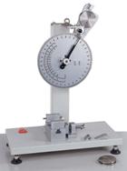
Example 3: The Charpy Impact Test is a way to measure the work of fracture of a material (i.e. the work per unit area required to separate a material into two pieces). An example (from www.qualitest-inc.com/qpi.htm) is shown in the picture. You can see one in Prince Lab if you are curious.
It consists of a pendulum, which swings down from a prescribed initial angle to strike a specimen. The pendulum fractures the specimen, and then continues to swing to a new, smaller angle on the other side of the vertical. The scale on the pendulum allows the initial and final angles to be measured. The goal of this example is to deduce a relationship between the angles and the work of fracture of the specimen.
 The figure shows the pendulum before and after it hits
the specimen.
The figure shows the pendulum before and after it hits
the specimen.
- The potential energy of the mass before it is
released is . Its kinetic energy is zero.
- The potential energy of the mass when it comes to
rest after striking the specimen is . The kinetic energy is again zero.
The work of fracture is equal to the change in potential energy -
Example 4: Estimate the maximum distance that a long-bow can fire an arrow.
We can do this calculation by idealizing the bow as a spring, and estimating the maximum force that a person could apply to draw the bow. The energy stored in the bow can then be estimated, and energy conservation can be used to estimate the resulting velocity of the arrow.
Assumptions
- The long-bow will be idealized as a linear spring
- The maximum draw force is likely to be around 60lbf (270N)
- The draw length is about 2ft (0.6m)
- Arrows come with various masses typical range is between 250-600 grains (16-38 grams)
- We will neglect the mass of the bow (this is not a very realistic assumption)
Calculation: The calculation needs two steps: (i) we start by calculating the velocity of the arrow just after it is fired. This will be done using the energy conservation law; and (ii) we then calculate the distance traveled by the arrow using the projectile trajectory equations derived in the preceding chapter.
- Just before the arrow is released, the spring is
stretched to its maximum length, and the arrow is stationary. The total energy of the system is , where L is the draw length and k is the stiffness of the bow.
- We can estimate values for the spring stiffness
using the draw force: we have that , so. Thus.
- Just after the arrow is fired, the spring returns
to its un-stretched length, and the arrow has velocity V. The total energy of the system
is , where m is the mass of the arrow
- The system is conservative, therefore
- We suppose that the arrow is launched from the
origin at an angle to the horizontal. The horizontal and vertical components of velocity are. The position vector of the arrow can be calculated using the method outlined in Section 3.2.2the result is
We can calculate the distance traveled by noting that its position vector when it lands is di. This gives
where t is the time of flight. The i and j components of this equation can be solved for t and d, with the result
The
arrow travels furthest when fired at an angle that maximizes - i.e. 45
degrees. The distance follows as
- Substituting numbers
gives 2064m for a 250 grain arrow over a mile! Of course air resistance will reduce this value, and in practice the kinetic energy associated with the motion of the bow and bowstring (neglected here) will reduce the distance.
 Example 5: Find a formula for the escape velocity of a space
vehicle as a function of altitude above the earths surface.
Example 5: Find a formula for the escape velocity of a space
vehicle as a function of altitude above the earths surface.
The
term ‘Escape velocity’ means that the space vehicle has a large enough velocity
to completely escape the earth’s gravitational field i.e. the space vehicle will never stop after
being launched.
Assumptions
- The space vehicle is initially in orbit at an altitude h above the earth’s surface
- The earth’s radius is 6378.145km
- While in orbit, a rocket is burned on the vehicle to increase its speed to v (the escape velocity), placing it on a hyperbolic trajectory that will eventually escape the earth’s gravitational field.
- The Gravitational parameter (G= gravitational constant; M=mass of earth)
Calculation
- Just after the rocket
is burned, the potential energy of the system is , while its kinetic energy is
- When it escapes the earth’s gravitational field (at an infinite height above the earth’s surface) the potential energy is zero. At the critical escape velocity, the velocity of the spacecraft at this point drops to zero. The total energy at escape is therefore zero.
- This is a conservative system, so
- A typical low earth orbit has altitude of 250km. For this altitude the escape velocity is 10.9km/sec.
4.1.11 Force, Torque and Power curves for actuators and motors
Concepts of power and work are particularly useful to calculate the behavior of a system that is driven by a motor. Calculations like this are described in more detail in Section 4.12. In this section, we discuss the relationships between force, torque, speed and power for motors.
There are many different types of motor, and each type has its own unique characteristics. They all have the following features in common, however:
- The motors convert some non-mechanical form of energy into mechanical work. For example, an electric motor converts electrical energy; an internal combustion engine, your muscles, and other molecular motors convert chemical energy, and so on. You may be interested in an extensive discussion of muscles at http://www.unmc.edu/physiology/Mann/mann14.html
- A linear motor or linear actuator applies a force to an object (or more accurately, it applies roughly equal and opposite forces on two objects connected to its ends). Your muscles are good examples of linear actuators. You can buy electrical or hydraulically powered actuators as well.
- The forces applied by an actuator depend on (i) the amount of power
supplied to the actuator electrical, chemical, etc; and (ii) the rate of contraction, or stretching, of the actuator. The typical variation of force with stretch rate is shown in the figure. The figure assumes that the actuator pulls on the objects attached to its ends (like a muscle); but some actuators will push rather than pull; and some can do both. If the actuator extends slowly and is not rotating it behaves like a two-force member, and the forces exerted by its two ends are equal and opposite.
- A rotary motor or rotary
actuator applies a moment or
torque to an object (or, again,
more precisely it applies
equal
and opposite moments to two objects).
Electric motors, internal combustion engines, bacterial motors are
good examples of rotary motors.
- The torques exerted by
a rotary actuator depend on (i) the amount of power supplied to the
actuator electrical, chemical, etc; and (ii) the relative velocity of the two objects on which the forces act. The typical variation of force with external power applied and with relative velocity is shown in the figure. An electric motor applies a large torque when it is stationary, and its torque decreases with rotational speed. An internal combustion engine applies no torque when it is stationary. It’s torque is greatest at some intermediate speed, and decreases at high speed.
The
power
curve describes the variation of the rate of work done by an actuator
or motor with its extension or contraction rate or rotational speed. Note that
- The rate of work done
(or power expended) by a linear actuator that applies forces ,to the objects attached to its two ends can be calculated as, whereandare the velocities of the two ends.
- The rate of work (or
power expended) by a rotational motor that applies moments ,to the objects attached to its two ends is.
Typical
power curves for motors and actuators are sketched in the figures.
The
efficiency
of a motor or actuator is the ratio of the rate of work done by the forces or
moments exerted by the motor to the electrical or chemical power. The efficiency is always less than 1 because
some fraction of the power supplied to the motor is dissipated as heat. An electric motor has a high efficiency; heat
engines such as an internal combustion engine have a much lower efficiency,
because they operate by raising the temperature of the air inside the cylinders
to increase its pressure. The heat
required to increase the temperature can never be completely converted into
useful work (EN72 will discuss the reasons for this in more detail). The efficiency of a motor always varies with
its speed there is a special operating speed that
maximizes its efficiency. For an
internal combustion engine, the speed corresponding to maximum efficiency is
usually quite low
1500rpm or so.
So, to minimize fuel consumption during your driving, you need to
operate the engine at this speed for as much of your drive as possible.
There
is not enough time in this course to be able to discuss the characteristics of
actuators and motors in great detail.
Instead, we focus on one specific example, which helps to illustrate the
general characteristics in more detail.
Torque
Curves for a brushed electric motor. There are several different types of electric motor here, we will focus on the simplest and
cheapest
the so called `
Here
is a very brief summary of the basic principles of this type of motor. The underlying theory will be discussed in
more detail in EN510
![]() An electric motor applies a moment, or torque to an object that is
coupled to its output shaft. The moment
is developed by electromagnetic forces acting between permanent magnets in the
housing and the electric current flowing through the winding of the motor. In the following discussion, we shall assume
that the body of the motor is stationary
An electric motor applies a moment, or torque to an object that is
coupled to its output shaft. The moment
is developed by electromagnetic forces acting between permanent magnets in the
housing and the electric current flowing through the winding of the motor. In the following discussion, we shall assume
that the body of the motor is stationary ,
and its output shaft rotates with angular velocity
where n
is a unit vector parallel to the shaft and
is its angular speed. In addition, we assume that the output shaft
exerts a moment
.
![]() Power to drive the motor is supplied by
connecting an electrical power source (e.g. a battery) to its terminals. The power supply generally applies a fixed voltage to the terminals, which then
causes current to flow through the winding.
The current is proportional to the voltage, and decreases in proportion
to the angular (rotational) speed of the output shaft of the motor.
Power to drive the motor is supplied by
connecting an electrical power source (e.g. a battery) to its terminals. The power supply generally applies a fixed voltage to the terminals, which then
causes current to flow through the winding.
The current is proportional to the voltage, and decreases in proportion
to the angular (rotational) speed of the output shaft of the motor.
![]() The moment applied by the output shaft is
proportional to this electric current.
The moment applied by the output shaft is
proportional to this electric current.
The
electric current I flowing through
the winding is related to the voltage V
and angular speed of the motor (in radians per second) by
where
R is the electrical resistance of the
winding, and is a constant that depends on the arrangement
and type of magnets used in the motor, as well as the geometry of the wire
coil.
The
magnitude of moment exerted by output shaft of the motor T is related to the electric current and the speed of the motor by
where
and
are constants that account for losses such as
friction in the bearings, eddy currents, and air resistance.
The
torque-current and the current-voltage-speed relations can be combined into a
single formula relating torque to voltage and motor speed
 This relationship is sketched in the figure
 this is called the torque curve for the
motor. The two most important points on
the curve are
- The `stall torque’
- The `No load’ speed
The
torque curve can be expressed in terms of these quantities as
Motor
manufacturers generally provide values of the stall torque and no load speed
for a motor. Some manufacturers provide
enough data so that you can usually calculate the values of R, ,
and
for their product. For example, a very detailed set of motor
specs are shown in the table below. The
table is from http://www.motortech.com/dcmotorCIR_MD.htm Each row of the table refers to a different
motor.
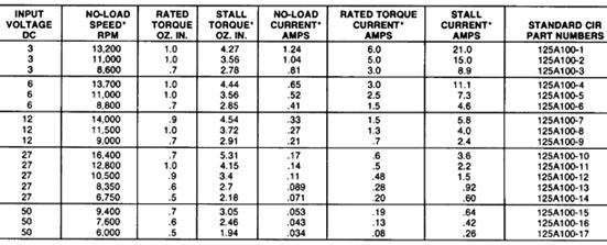
Here
- The `input voltage’ is
the recommended voltage V to
apply to the motor. All other data
in the table assume that the motor is used with this voltage. If you wish,
you can run a motor with a lower voltage (this will make it run more
slowly) and if you are feeling brave you can increase the voltage slightly
but this might cause it to burn out, invalidate your warranty and expose you to a potential lawsuit from your customers…
- The `No load speed’ is the speed of the motor when it is spinning freely with T=0
- The `No load current’ is the corresponding current
- The `Stall torque’ is the value of T when the motor is not spinning
- The ‘Stall current’ is the corresponding current
- The `rated torque’ and
`rated current’ are limits to the steady running of the motor the torque and current should not exceed these values for an extended period of time.
The
values in the table can be substituted into the formulas relating current,
voltage, torque and motor speed, which yield four equations for the unknown
values of R, ,
and
Solving
these equations gives
HEALTH WARNING: When you use these formulas it is critical to use a
consistent set of units. SI units are very
strongly recommended! Volts and Amperes
are SI units of electrical potential and electric current. But the torques must be converted into Nm. The conversion factor is 1 ‘oz-in’ is
0.0070612 Nm.
Not
all motor manufacturers provide such detailed specifications it is more common to be given (i) the stall
torque; (ii) the no load speed; and (iii) the stall current. If this is the case you have to assume
and take
. If you aren’t given the stall current you
have to take
as well.
 Power Curves for a brushed electric motor driven from
a constant voltage power supply: The
rate of work done by the motor is
Power Curves for a brushed electric motor driven from
a constant voltage power supply: The
rate of work done by the motor is . The power can be calculated in terms of the
angular speed of the motor as
The
power curve is sketched in the figure.
The most important features are (i) The motor develops no power at both
zero speed and the no load speed; and (ii) the motor develops its maximum power
at speed
.
Efficiency of a brushed electric motor: The electrical power supplied to a motor can be
calculated from the current I and
voltage V as . The efficiency can therefore be calculated
as
The second expression can be
used to calculate the speed that maximizes efficiency.
4.1.12 Power transmission in machines
A machine is a system that converts one
form of motion into another. A lever is a
simple example if point A on the lever is made to move, then
point B will move either faster or slower than A, depending on the lengths of
the two lever arms. Other, more
practical examples include
 Your
skeleton; used to help convert muscle motion into various more useful
forms…
Your
skeleton; used to help convert muscle motion into various more useful
forms…- The transmission of a
vehicle used to convert rotational motion induced by the engine’s crank-shaft to translational motion of the vehicle
- A gearbox converts rotational motion at one angular speed to rotational motion at another.
- A system of pulleys.
Concepts
of work and energy are extremely useful to analyze transmission of forces and
moments through a machine. The goal of
these calculations is to quickly determine relationships between external
forces acting on the machine, rather than to analyze the motion of the
system itself.
To
do this, we usually make two assumptions:
- The machine is a
conservative system. This is true
as long as friction in the machine can be neglected.
- The kinetic and
potential energy of the mechanism within the machine can be neglected. This is true if either (i) the machine
has negligible mass and is very stiff (i.e. it does not deform); or (ii)
the machine moves at steady speed or is stationary.
If
this is the case, the total rate of work
done by external forces acting on the machine is zero. This principle can be used to relate external
forces acting on the machine, without having to work through the very lengthy
and tedious process of computing all the internal forces.
The
procedure to do this is always:
- Derive a relationship
between the velocities of the points where external forces act this is always a geometric relationship.
- Write down the total
rate of external work done on the system
- Use (1) and (2) to
relate the external forces to each other.
The
procedure is illustrated using a number of examples below.
Example 1: As a first example, we derive a formula relating the
forces acting on the two ends of a lever. Assume that the forces act
perpendicular to the lever as shown in the figure.
Calculation
- Suppose that the lever
rotates about the pivot at some angular rate .
- The ends of the lever
have velocities (see the circular motion example in the preceding chapter if you can’t remember how to show this.
- The force vectors can
be expressed as
- The reaction forces at
the pivot are stationary and so do no work.
- The total rate of work done on the lever is
therefore
- The rate of external work is zero, so
Example 2: Here we revisit an EN3 statics problem. The rabbit uses a pulley system to raise
carrot with weight W. Calculate the force applied by the rabbit on
the cable.
- The velocity of the
end of the cable held by the rabbit is , with direction parallel to the cable
- The velocity of the
carrot is ; its direction is vertical
- The total length of
the cable (aside from small, constant lengths going around the pulleys) is
. Since the length is constant, it follows that
- The external forces
acting on the pulley system are (i) the weight of the carrot W, acting vertically; (ii) the unknown
force F applied by the rabbit,
acting parallel to the cable; and (iii) the reaction force acting on the
topmost pulley. The rate of work done by the rabbit is , the rate of work done by the gravitational force acting on the carrot is. The reaction force is stationary, and so does no work. The total rate of work done is therefore
- Using (3) and (4) we see that
Example 3 Calculate the torque that must be applied to a screw
with pitch d in order to raise a
weight W.
Here,
we regard the screw as a machine subjected to external forces.
- When the screw turns
through one complete turn ( radians) it raises the weight by a distance d
- The work done by the
torque is ; the work done by the weight isWd. The reaction forces acting on the thread of the screw do no work
- The total work is
zero, therefore .
 Example 4: A gearbox is used for two purposes: (i) it can amplify
or attenuate torques, or moments; and (ii) it can change the speed of a
rotating shaft. The characteristics of a gearbox are specified by its gear ratio specifies the ratio of the rotational speed of the output
shaft to that of the input shaft
Example 4: A gearbox is used for two purposes: (i) it can amplify
or attenuate torques, or moments; and (ii) it can change the speed of a
rotating shaft. The characteristics of a gearbox are specified by its gear ratio specifies the ratio of the rotational speed of the output
shaft to that of the input shaft .
The
sketch shows an example. A power source
(a rotational motor) drives the input shaft; while the output shaft is used to
drive a load. The rotational motion of
the input and output shafts can be described by angular velocity vectors (note that the
shafts don’t necessarily have to rotate in the same direction
if they don’t then one of
will be
negative).
A
quick power calculation can be used to relate the moments acting on the
input and output shafts.
- The gear ratio relates
the input and output angular velocities as
- The rate of work done
on the gearbox by the moment acting on the input shaft is . The work done by the moment acting on the output shaft is. A reaction moment must act on the base of the gearbox, but since the gearbox is stationary this reaction moment does no work.
- The rate of work done by all the external forces on the gearbox is zero, so
 Example 5: Find a formula for the engine power required for a
vehicle with mass m to climb a slope
with angle
Example 5: Find a formula for the engine power required for a
vehicle with mass m to climb a slope
with angle at speed v.
Estimate values for engine power required for various vehicles to climb a
slopes of 3%, 4% and 5% (these are typical standard grades for flat, rolling
and mountain terrain freeways, see, e.g. the Roadway Engineering Highway Design
Manual for Oregon at http://www.oregon.gov/ODOT/HWY/ENGSRVICES/hwy_manual.shtml#2003_English_Manual
Also,
estimate (a) the torque exerted by the engine crankshaft on the transmission;
and (b) the force acting on the pistons of the engine.
Assumptions:
- The only forces acting
on the vehicle are aerodynamic drag, gravity, and reaction forces at the
driving wheels.
- Aerodynamic drag will
be assumed to be in the high Reynolds number regime, with a drag
coefficient of order
- The crankshaft rotates
at approximately 2000rpm.
- As a representative
examples of engines, we will consider (i) a large 6 cylinder 4 stroke
diesel engine, with stroke (distance moved by the pistons) of 150mm; and
(ii) a small 4 cylinder gasoline powered engine with stroke 94mm
(see http://www.automotive.com/2009/12/chevrolet/cobalt/specifications/index.html)
 Calculation.
The figure shows a free body diagram for the truck. It shows (i) gravity; (ii) Aerodynamic drag;
(iii) reaction forces acting on the wheels.
Calculation.
The figure shows a free body diagram for the truck. It shows (i) gravity; (ii) Aerodynamic drag;
(iii) reaction forces acting on the wheels.
- The velocity vector of
the vehicle is
- The rate of work done by the gravitational and aerodynamic forces is
where
,
with
the drag coefficient, A the frontal area of the
vehicle, and
the air density.
- The reaction forces
acting on the wheels do no work, because they act on stationary points
(the wheel is not moving where it touches the ground).
- The kinetic energy of
the vehicle is constant, so the total rate of work done on the vehicle
must be zero. The moving parts of the engine (specifically, the pressure acting on the pistons) do
work on the vehicle. Denoting the
power of the engine by , we have that
- The torque exerted by
the crankshaft can be estimated by noting that the rate of work done by
the engine is related to the torque T
and the rotational speed of the crankshaft by. The torque follows as
- The force F on the pistons can be estimated
by noting that the rate of work done by a piston is related to the speed
of the piston v by . In a four-stroke engine, each piston does work 25% of the time (during the firing stroke). If the engine has n cylinders, the total engine power is therefore. Finally, the piston speed can be estimated by noting that the piston travels the distance of the stroke during half a revolution, and so has average speed. This shows that.
The
table below calculates values for two examples of vehicles
|
Vehicle |
Grade |
Weight (kg) |
Frontal area
|
Drag |
Speed |
Engine Rad/sec |
Stroke m |
Engine power |
Torque Nm |
Piston force N |
|
18 wheeler |
3% |
36000 |
10 |
0.1 |
29 |
12600 |
0.15 |
320000 |
25 |
355 |
|
4% |
420000 |
34 |
470 |
|||||||
|
5% |
520000 |
42 |
580 |
|||||||
|
Chevy |
3% |
1250 |
2.5 |
.1 |
29 |
12600 |
0.095 |
14000 |
1.1 |
36 |
|
4% |
17000 |
1.4 |
46 |
|||||||
|
5% |
21000 |
1.7 |
55 |