
EN4: Dynamics and Vibrations
Division of Engineering
Brown University
A rigid body is an idealization of a body that does not deform or change shape. Formally it is defined as a collection of particles with the property that the distance between particles remains unchanged during the course of motions of the body. Like the approximation of a rigid body as a particle, this is never strictly true. All bodies deform as they move. However, the approximation remains acceptable as long as the deformations are negligible relative to the overall motion of the body.
Figure 5.1: Deformations experienced by an aircraft are small relative to its motion.
As an example, the flutter of an aircraft wing during the course of a flight is clearly negligible relative to the motion of the aircraft as a whole. On the other hand, if one was interested in stresses induced in the wing as a consequence of the flutter, these deformations become of primary importance.
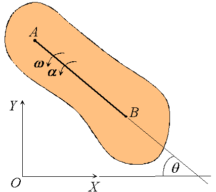
Figure 5.2: Schematic showing a planar rigid body.
In the following, we will restrict attention to the planar motion of rigid bodies. In particular, we will take all rigid bodies to be thin slabs with motion constrained to lie within the plane of the slab. Unless otherwise indicated, we will assume basis vectors of the form {i, j, k}, such that i and j lie in the plane, with k is the plane normal.
5.1 Kinematics of Rigid Body Motion
In the following we will derive expressions that describe the general motion of a rigid body in the plane. As rigid bodies are viewed as collections of particles, this may appear an insurmountable task, requiring a description of the motion of each particle. However, the assumption that the body does not deform is a very strong one, requiring that the distance between every pair of particles comprising the body remains unchanged. To satisfy this, the particles that comprise a rigid body must move in concert, making the kinematics almost trivial.
Before we can proceed to this, however, we need to be able to analyze motion relative to a set of translating axes.
5.1.1 Preliminaries: Motion Relative to Translating Axes
In the course so far particle motion has been described using position vectors that were referred to fixed reference frames. The positions, velocities and accelerations determined in this way are referred to as absolute. Often it isn’t possible or convenient to use a fixed set of axes for the observation of motion. Many problems are simplified considerably by the use of a moving reference frame.
In the following we will restrict our attention to moving reference frames that translate but do not rotate.
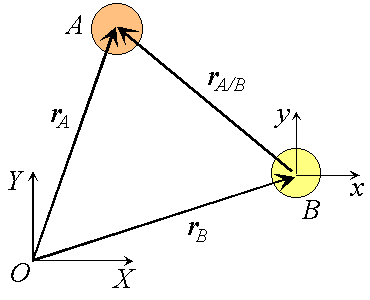
Figure 5.1.1: Observation of particle motion using a translating reference.Consider two particles A and B moving along independent trajectories in the plane, and a fixed reference O. Let
and
be the positions of particles A and B in the fixed reference. Instead of observing the motion of particle A relative to the fixed reference as we have done in the past, we will attach a non-rotating reference to particle B and observe the motion of A relative to the moving reference at B. Let i and j be basis vectors of the moving reference, then the position vector of A relative to the reference at B, denoted
is,
where the subscript stands for "A with respect to B" or "A relative to B". Observe that, as the moving frame does not rotate, basis vectors i and j do not change in time. Therefore, taking time derivatives, we obtain simply,
which can be interpreted as the velocity of A relative to B. Now we can express the absolute position vector of A as,
Differentiating the equation in time to obtain expressions for the absolute velocity and acceleration of particle A:
or the absolute velocity of A equals the absolute velocity of B plus the velocity of A relative to B,
, and similarly for the acceleration. The relative terms are the velocity or acceleration measured by an observer attached to the moving reference at particle B.
Figure 5.1.2: Relative velocities under change of translating reference.
What would happen if the moving reference were attached to A instead?
By comparison with expressions derived previously:

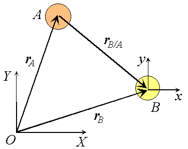


For motion relative to a translating reference:
which describe the motion of particle A observed relative to a translating reference at B. |

5.1.2 Properties of Rigid Body Motion
In the following, we identify two properties of the motion of rigid bodies that simplify the kinematics significantly. In order to do this, observe that an arbitrary rigid body motion falls into one of the three categories:
- Translation, rectilinear and curvilinear: Motion in which every line in the body remains parallel to its original position. The motion of the body is completely specified by the motion of any point in the body. All points of the body have the same velocity and same acceleration.
- Rotation about a fixed axis: All particles move in circular paths about the axis of rotation. The motion of the body is completely determined by the angular velocity of the rotation.
- General plane motion: Any plane motion that is neither a pure rotation nor a translation falls into this class. However, as we will see below, a general plane motion can always be reduced to the sum of a translation and a rotation.
We proceed by demonstrating that every motion of a planar rigid body is associated with a single angular velocity
and angular acceleration
, describing the angular displacement of an arbitrary line inscribed in the body relative to a fixed direction.
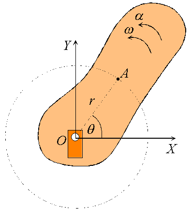
Figure 5.1.3: Angular velocity and acceleration of a rigid body.
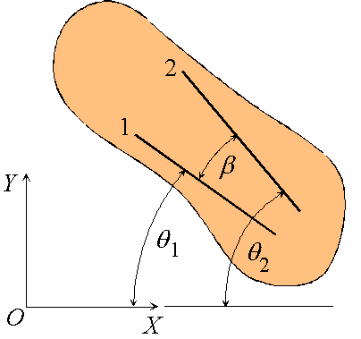
Consider a rigid body undergoing plane motion. The angular positions of two arbitrary lines 1 and 2 attached to the body are specified by
and
measured relative to any convenient fixed reference direction. These are related to the intermediate angle
shown as,
Observe that as the body is rigid, requiring that the distance between each pair of points on the two lines 1 and 2 is constant, angle
These hold for arbitrary lines attached to the body, implying in turn that the body can be associated with a unique angular velocity
for an arbitrary line attached to the body. Arguing analogously, the body can be associated with a unique angular acceleration
Figure 5.1.4: Angular velocity and angular acceleration of a rigid body.
Consequently, we have the property that all lines on a rigid body in its plane of motion have the same angular displacement, the same angular velocity
Figure 5.1.5: Decomposition of rigid body motion.
Next, consider the motion of a rigid body over the interval
as shown, with arbitrary point
taken as reference. Clearly, the motion can be consider to occur in two stages: a translation with reference
taking arbitrary line
to an intermediate position
; and a rotation about point
taking
. This corresponds to a decomposition of the motion into the sum of a translation and a rotation. While the translational motion is described by the velocity
and acceleration
of the reference point, the rotational motion is characterized by the unique angular velocity

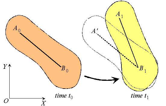
Characteristics of rigid body motion:
|
5.1.3 Governing Equations: Velocities and Accelerations
With this understanding of the structure of plane motion of rigid bodies, we are in a position to move onto the business of attempting to derive equations that describe the motion.
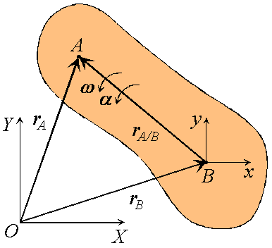
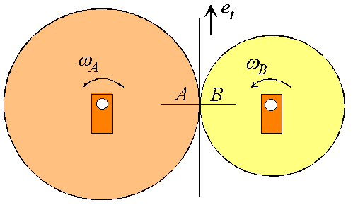
Figure 5.1.6: Definition of a translating reference attached to point B.
Consider a rigid body moving in the plane with angular velocity
and angular acceleration
, and two arbitrary points A and B of the body. We will examine the motion of this body in both, the fixed reference O shown, as well as relative to a non-rotating reference attached to point B. Proceeding, we express the absolute position of point A in terms of the absolute position of point B as,
where
where
is the velocity of point A relative to the reference at B,
Figure 5.1.7: Motion of point A as seen by a translating observer at B.
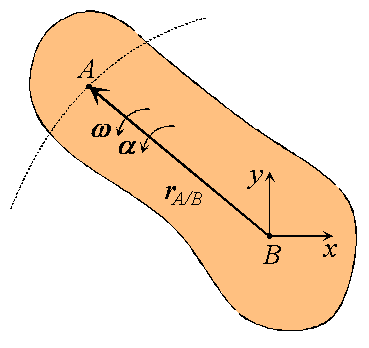
Now, as the body moves, point A traces a circular path of radius
relative to point B, keeping the distance between the two unchanged. The angular velocity of this motion is simply the angular velocity
or,
Observe that the expression reflects the decomposition of rigid body motion referred to previously. With B chosen as reference, the velocity of A is the vector sum of a translational portion
and a rotational portion
.
Proceeding to derive expressions for the acceleration of an arbitrary point of a rigid body, we differentiate the equation for velocities to obtain,
where
, the acceleration of point A relative to the reference at B, is simply
or,
Thus, like the absolute velocity, the absolute acceleration of point A is the vector sum of a translational portion
and a rotational portion
.
For arbitrary rigid body motion:
where |
5.1.4 Application: Fixed Axis Rotation
In the following we will apply the kinematical relations derived to the case of a rigid body rotating about a fixed axis. As will be seen, the relations will reduce to familiar forms once n-t coordinates are introduced.
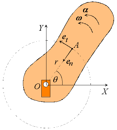
Figure 5.1.8: n-t coordinates for fixed axis rotation.
Consider an arbitrary point A of a rigid body rotating with angular velocity
and
be unit vectors tethered to point A as shown, with
and acceleration
of point A:
where
is the position vector of A relative to the axis. Now, as the motion is planar, the angular velocity and angular acceleration have the form,
Substituting these yields the simplified expressions,
or,
where
can be recognized as the normal or centripetal acceleration, and
is the tangential acceleration.
Figure 5.1.9: Velocities and accelerations associated with fixed axis rotation.
To help develop some intuition, we turn to examine the structure of the velocity and acceleration fields over the rotating body. For velocities we have simply,
or the velocity of a point in the body is perpendicular to the line connecting the point to the axis of rotation, with magnitude proportional to its distance from the axis. The acceleration, on the other hand, is composed of the two pieces:
while the centripetal acceleration is directed towards the axis, the tangential acceleration is along
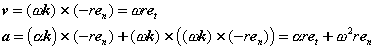
For the fixed axis rotation of a rigid body:
alternately,
where |
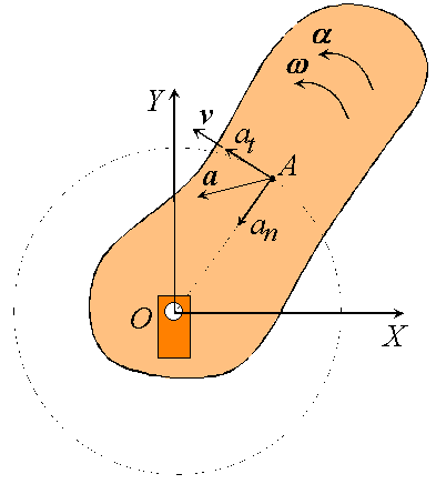
Caution: Angle Conventions
When working with n-t coordinates, care must be taken to ensure that a consistence choice of tangent vectors
is made as two conventions exist for rotational quantities
in the plane. The two differ in the first taking counter-clockwise rotations to be positive, which is recommended,
while the second takes clockwise rotations to be positive:
Figure 5.1.10: Alternate angular conventions for use with planar rotations.
In either case,
.
Aside: Describing Rotational Motion
Figure 5.1.11: Polar coordinates describing the position of point A.
Observe that when polar coordinates
are used, the coordinates of a point of a rotating body are determined by its angular displacement
Therefore, in order to describe the motion of A, all that is necessary is a determination of
and angular acceleration
describe the rotation of any line in the body, we have the relations
Given
, therefore, techniques developed previously can be applied to integrate these to determine
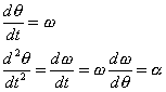
5.1.5 Application: Rigid Bodies in Contact
We proceed now to develop techniques to analyze the motion of rigid bodies in contact. We consider two contacting rigid bodies, and assume that no sliding occurs at the contacting surfaces. Let A and B be points, one on each of the rigid bodies, instantaneously in contact. As contact takes place without slipping, the velocity of A relative to B must vanish, or
where
and
are the absolute velocities of A and B, respectively.
Case I: Contact with another rotating rigid body
Figure 5.1.12: Rotating rigid bodies in contact.
An example of this form of contact is that between gears in a gear train: spur, bevel, helical or worm gears. In our consideration of planar motion, however, we are limited to analyzing contact between gears that have a common axis of rotation.
Consider the motion of instantaneously contacting points A and B, each on one of a pair of interlocking gears. Applying our contact relationship to A and B, we have
or,
However, as
we have,
where
,
and
,
are the radii and angular velocities of the two gears, respectively. Taking time derivatives, we obtain a relationship between the accelerations of points A and B,
or the two points have tangential accelerations of equal magnitude. Rearranging,
or the ratio of angular velocities of a pair of gears is inversely proportional to the ratio of their radii.
Case II: Contact with a translating body
Figure 5.1.13: A rotating rigid body in contact with a translating one.
Contact of this form is encountered in belt, rope, and chain drives of all kinds, as well as between rack and pinion gears.
As before, consider the motion of instantaneously contacting points, A on the rotating body, and B on the translating one. As the two points must have identical absolute velocities, the velocity of point B must be directed along
, tangent to the path of A. Additionally,
and differentiating for a relationship linking the accelerations,
5.1.6 Application: General Plane Motion
With the case of planar fixed axis rotation dealt with, we turn now to the more complex situation of general plane motion. Recall, once again, that the motion of an arbitrary rigid body can be reduced to the superposition of a translation and a fixed axis rotation. Handling the translation of a rigid body is trivial, all points of the body move with the same velocity and acceleration, and we now know how to deal with fixed axis rotations. Therefore, all that remains is to understand how the two are superposed. As we will find out, this is quite simple.
We proceed by returning to the equations we had derived for the arbitrary motion of a rigid body. Recall that these related the velocity
and acceleration
of a point A in the body to the translational motion of an arbitrary reference point B (
and
As in the case of fixed axis rotation we simplify these expressions by introducing a set of n-t coordinates. Unlike those used previously, however, the coordinates introduced here refer to the motion of A relative to the reference at B. Therefore,
is directed towards point B, the center of the relative motion, and
is directed along
, tangent to the path of A relative to B.
Figure 5.1.14: n-t coordinates for general plane motion.
Substituting, we obtain a simplified expression for the velocity of point A,
which can be recognized as a superposition of translational and rotational components, each of which we understand very well.
Figure 5.1.15: Decomposition of the absolute velocity of point A.
Proceeding in an analogous way for the acceleration,
or,
with normal and tangential accelerations of the form,
Therefore, like the velocity, the acceleration of A is a superposition of translational and rotational components. While the normal component is directed along
Figure 5.1.16: Decomposition of the absolute acceleration of point A.


For the general plane motion of a rigid body:
alternately,
where |