|
Calibration Procedures
Data Processing
Calibration Procedures [top]
Through
the previous four-step DIY, you must be anxious to see how this simple
device can work on the sophisticated AFM system. Let's start with the demonstration by showing some of the videos I took using an optical microscope: side view , top view.
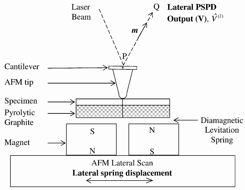
A schematic of the D-LFC is shown in Figure 7. In
the setup, the diamagnetic levitation system is
mounted on the stage of the AFM base scanner.
For the calibration, you just do the normal LFM measurement; the only
thing different is that your sample is now replaced by the D-LFC. Once
the AFM tip is engaged on the PG composite surface, the
magnets together with the AFM base are reciprocated by the lateral
scanner,
while the normal load is held fixed by
holding the normal PSPD output  constant through the
feedback controller. It
should be noticed that we used the Park Scientific Instrument AutoCP
AFM system. For those systems with a fixed sample holder but a moving
probe, the magnets are stationary while the PG sheet moves together with
the probe after the engagement. constant through the
feedback controller. It
should be noticed that we used the Park Scientific Instrument AutoCP
AFM system. For those systems with a fixed sample holder but a moving
probe, the magnets are stationary while the PG sheet moves together with
the probe after the engagement.
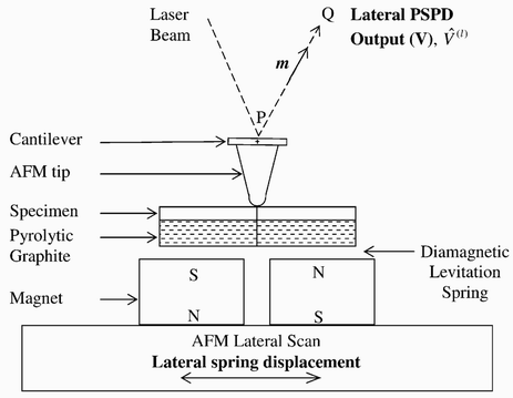
Figure 7. A schematic of the D-LFC
The lateral PSPD output  is recorded against the lateral base displacement is recorded against the lateral base displacement  . The displacement is related to the lateral force . The displacement is related to the lateral force  by by
 (5) (5)
where the base displacement can be decomposed 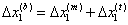 , into the displacements of the magnetic spring , into the displacements of the magnetic spring  and the AFM tip and the AFM tip  . The tip displacement is caused by the
compliance of the tip contact and the cantilever twist. It is typically within
a few nanometers while the magnetic spring displacement is on the order of tens
of micrometers. Therefore, the tip displacement can be neglected in (5). In this calibration procedure, the maximum
reciprocating displacement of the lateral base displacement . The tip displacement is caused by the
compliance of the tip contact and the cantilever twist. It is typically within
a few nanometers while the magnetic spring displacement is on the order of tens
of micrometers. Therefore, the tip displacement can be neglected in (5). In this calibration procedure, the maximum
reciprocating displacement of the lateral base displacement  is limited to induce a
lateral force well within the static
friction force of the onset of slip. is limited to induce a
lateral force well within the static
friction force of the onset of slip.

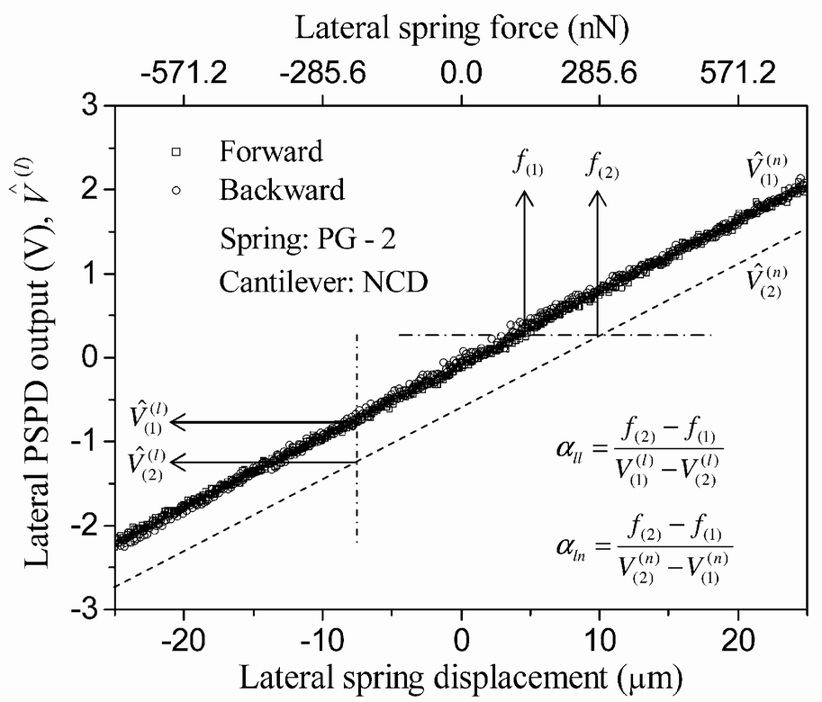
Figure 8. A diagram showing the D-LFC principles for measuring the AFM force constants
Figure 8 shows an experimental measurement of the lateral PSPD output
against the lateral displacement of the magnets on the AFM base reciprocated
within 25 µm for contact between a
mica specimen mounted on a levitated PG sheet and a spherical
bead attached near the end of an AFM cantilever.
The bead is made of boro-silicate glass coated with a 50 nm gold layer and has
a diameter of 15 µm. The experimental data show that the response is linear and
reversible within the thermal and feed-back noise band for forward and backward
scanning of the base displacement.
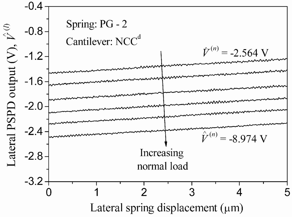
Step-1:
Use the D-LFC as your sample and collect the LFM data as normal.
Multiple data sets should be collected for different normal loads
(usually called set point) if you want the crosstalk force constant to
be calibrated.
If everything is carried out correctly, you will get the data similar to those shown in Figure 9.
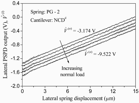
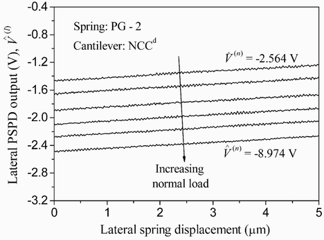
Figure 9. D-LFC data of the lateral PSPD output under incremental normal loads
According
to our experiences, this is the trickiest part of the calibration
process. Here are some tips, you may find them useful (or you can
contact me if you have some other weird problems):
- Use a larger scan size, i.e. larger spring displacement, as long as the probe doesn't slip relatively to the PG surface;
- Put
an acoustic cover if your AFM system has one; because the PG sheet is
floating in air, it is susceptible to the acoustic noise; and if your system has a poor vibration isolation, you can try the data averaging if necessary;
- If
you observe a significant oscillation in vertical direction, that's due
to the setting of feedback parameters; play with them you should be
able to find the recipe for your own AFM system. The reason for this is
that the feedback circuit could behave like an extra "electric spring"
to make the D-LFC and your probe at around resonant status;
- Use a reasonable
slow scan rate; this would reduce the effect of the eddy current and the
possible air perturbation, though our testing shows that the
calibration results are not sensitive to them.
Data Processing [top]
The data processing is summarized in Figure 8.
To simplify data processing, the AFM base displacement is approximated
as the lateral spring displacement. Then it is multiplied by the spring
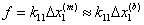
constant  and converted to the lateral force , which is shown on the horizontal
axis at the top of Fig. 8. Now we have a data set relating and for a fixed value of . Recalling the equation (1) in Background in a difference form,
and converted to the lateral force , which is shown on the horizontal
axis at the top of Fig. 8. Now we have a data set relating and for a fixed value of . Recalling the equation (1) in Background in a difference form,
  (6) (6)
the inverse slop,  , of the data is the lateral force constant , of the data is the lateral force constant  . In addition, two response lines for two different 's should be parallel to each other as shown by a dashed line in the figure. The crosstalk lateral force constant . In addition, two response lines for two different 's should be parallel to each other as shown by a dashed line in the figure. The crosstalk lateral force constant  is given by is given by  . Thus, experimental measurements of the responses 's with respect to the lateral force (or spring displacement) for two different 's can provide the values of both and via two linear fittings. . Thus, experimental measurements of the responses 's with respect to the lateral force (or spring displacement) for two different 's can provide the values of both and via two linear fittings.
Up to here, you have gone through all the details of D-LFC. Hope you enjoy this scientific toy :)
If you have any questions or comments, please don't hesitate to contact us.
|