
See previous file. Wk is a weight in a neural network. The formula can be seen as the Least Means Square approximation to true gradient descent. E is an "energy" or error function.
Feb 22, 1995 and forward, from EN291S, reformatted 2005
See chapter 4 of Simon Haykin, Neural Networks: A Comprehensive Foundation, 2nd Ed, Prentice-Hall, Upper Saddle River, NJ (1999) pp 161 ff.
And try Murray Smith's book, Neural Networks for Statistical Modeling, Van Nostrand Reinhold, 1993, ISBN 0-442-01310-8, QA76.87.S62
First: believe in gradient descent! What is it? 
See previous file. Wk is a weight in a neural network. The
formula can be seen as the Least Means Square approximation to true gradient
descent. E is an "energy" or error function.
In principle, a 2-layer BP network is complicated enough to solve
any (reasonable) classification problem, given enough time and precision. (time
for learning, and precision of weight resolution in the computer) Why? Because the
hidden layer presents various nonlinear compression functions to be combined at
the output layer. Each compression function is weighted and biased. The weight may
be negative or positive. The combining of the weights has similarities to Fourier
or Laplace transforms: representing something important with something convenient.
What do the biases do? provides an offset...
future GRAPHIC: COMPRESSION FUNCTIONS
For any weight in the 2-layer network, ![]() is all you need to compute, in principle, to obtain "instantaneous" weight
updates.
is all you need to compute, in principle, to obtain "instantaneous" weight
updates.
In simulating a 2-layer back prop a forward pass computes the hidden and output layer neuron responses. These responses are then used in a backward pass which updates the weights.
Notation
Haykin's notation is reasonable if you need something for an arbitrary number
of layers, but here we use a more direct notation to find hidden unit weight update
rules for a strict 2-layer system.
The only choice the designer normally has (and it's a big
choice) is the number of hidden units, J, below. Inputs K and outputs I are
usually fixed by the nature of the problem. What follows is notation a method
to update all weights by back propagation of error.
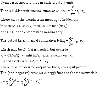
Furthermore, η is the learning rate for back prop.
Later we may also use superscript μ to denote which input pattern
is being presented.
BP weight update for output layer
Here we derive the update rule for the output layer weights in back prop, for
one pattern x, the components of which are the input xk's.
The weights for the ouput layer are the Wij's; we want a particular i & j
to update, so we need to compute
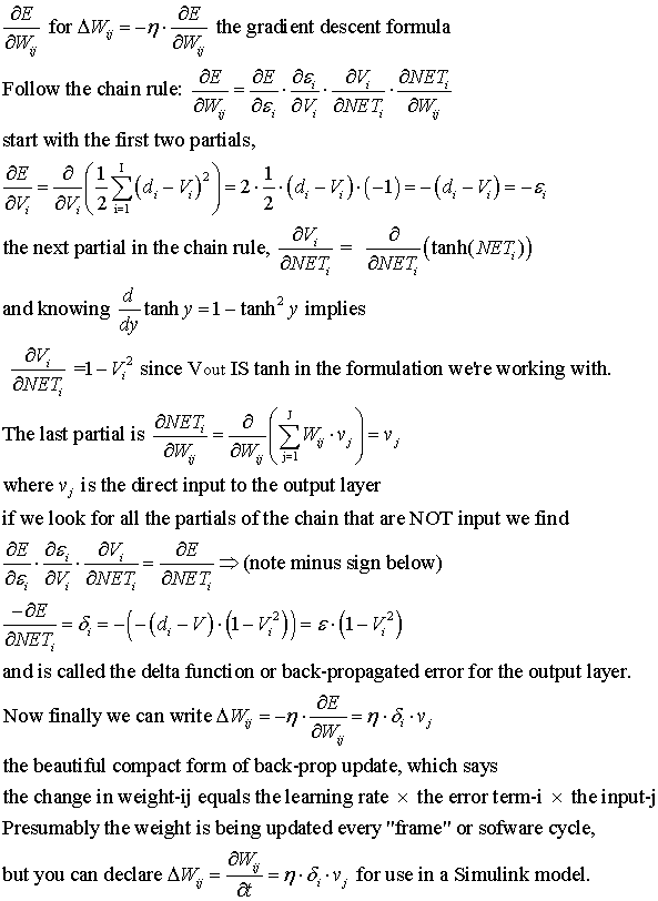
The d-V term is set up to appear as negative feedback.
Updating hidden layer weights
Consider hidden layer weight wjk where j is the hidden layer
index and k is the input index. We want
 (eqn **)
Here comes a critical concept to grasp. See figure below.
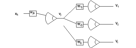
Notice that in a fully connected 2-layer network, hidden unit weight wjk
affects all the outputs V, through hidden unit output vj
projecting to output layer weights Wmj, m = 1,2, ..., I .
Examine

to verify that any Vm will involve a particular vj.
therefore the partial in equation ** above on all the δ-i's of the output
layer. Write out
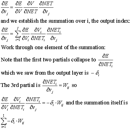
.
This development get us up to needing
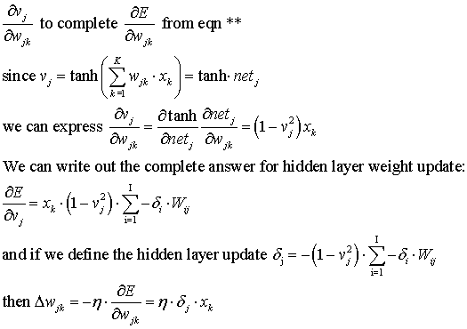
We're done! We have two formulas, one for updating the output layer, the other for
updating the hidden layer weights, pattern by {xk}μ pattern.
Do we need to know HU outputs in order to update by BP? Yes, and they're computed on the forward pass!
Implementing back prop with the Matlab Neural Network toolbox.
Using MATLAB you can efficiently implement the back prop algorithm.
(Efficiently for number of instructions, maybe not so efficient for speed...)
Let's say you want a 2-layer network:
You the designer need to make some decisions...
How many hidden units?
What compression function?
Initialize weights
error stopping criteria
learning rate
back prop code from the Matlab Neural Network Toolbox
documentation (3/05)
Creating a Network (newff).
The first step in training a feedforward network is to create the network object.
The function newff creates a feedforward network. It requires four inputs and returns
the network object. The first input is an R by 2 matrix of minimum and maximum values
for each of the R elements of the input vector. The second input is an array containing
the sizes of each layer. The third input is a cell array containing the names of
the transfer functions to be used in each layer. The final input contains the name
of the training function to be used.
For example, the following command creates a two-layer network. There is one input vector with two elements. The values for the first element of the input vector range between -1 and 2, the values of the second element of the input vector range between 0 and 5. There are three neurons in the first layer and one neuron in the second (output) layer. The transfer function in the first layer is tan-sigmoid, and the output layer transfer function is linear. The training function is traingd (which is described in a later section).
net=newff([-1
2; 0 5],[3,1],{'tansig','purelin'},'traingd');
This command creates the network object and also initializes the weights and biases of the network; therefore the network is ready for training. There are times when you may want to reinitialize the weights, or to perform a custom initialization. The next section explains the details of the initialization process.
Initializing Weights (init). Before training a feedforward network, the weights and biases must be initialized. The newff command will automatically initialize the weights, but you may want to reinitialize them. This can be done with the command init. This function takes a network object as input and returns a network object with all weights and biases initialized.
Here is how a network is initialized (or reinitialized):
net = init(net);
Below is Matlab code for direct computation
of back-propagated errors in a time series prediction application:
while cnt < max_cnt % & ssE > accu
shuf = [shuffleDT([1:sze-2], sze-2) sze-1 sze];
eta_decay = eta*exp(-3*cnt/max_cnt);
for mm = 1:sze %:-1:1
nn = shuf(mm);
DELW = eta_decay*del(nn)*hist_tot(:,nn)';
WtBP = WtBP+DELW;
end
V = tanh(WtBP*hist_tot);
epsilon = des_tot-V;
del = epsilon.*(1-V.*V);
ssE = sumsqr(del); % sum squared error
cnt = cnt+1;
end
Batch learning (speed) vs one-pattern-at-a-time learning (accuracy)
Could use other methods (breeding algorithm) to search for optimal weights...