EN224: Linear Elasticity

  

 

Division of Engineering

    Brown University

 

 

7.8 Complex variable solutions to mixed boundary value problems – contact and crack problems

 

 

In this section, we outline complex variable solutions to various 2D elasticity problems.  As a preliminary step, we summarize another important result in complex variables, which is immensely useful in solving mixed boundary value problems.

 

7.8.1 The Hilbert Problem

 

 

 

The Hilbert problem can be stated as follows:  Find a function  that is analytic everywhere except along a line L, bounded at infinity, and satisfies

on the line L (here, the notation  signifies that we approach the line from one side or the other).

 

We start by finding a function that satisfies

 clearly needs to be multiple-valued, so we might try something like a log or a square root.  In fact, the function

with a branch cut as shown in the figure does the trick (X is called a Plemelj function).  To see this, note that we can write

Tracing a path starting at A- and ending at A+ (so we don’t cross the branch cut) decreases both  and  by , so there is no discontinuity in X(z) at A.  In contrast, tracing a path starting at B- and ending at B+ decreases  by  and leaves  unchanged.  Consequently, for any point that lies on L, we have that

so that

If we choose  we will evidently satisfy .  In fact, any function of the form , where  will also work, since P(z) is continuous across L. In particular, we can multiply  by powers of either  or  to alter either the singularities at the ends of L, and/or the behavior of the function at infinity.

 

 

The function X(z) gives us the key to solving the inhomogeneous Hilbert problem.  Starting with

we can divide by  to see that

and using the properties of X(z) we see that

Now, we already know that the solution to

is

 

so that

The most general solution then has the form

 

 

7.8.2 Contact Problems

A generic contact problem is illustrated in the figure.  We consider a rigid indenter, with prescribed profile f(x), which is subjected to a normal force .  If friction acts between the indenter and the half-space, a horizontal force  may also act on the indenter.  We seek linear elastic solutions with stresses of order 1/r at infinity.

 

 

All the solutions in this section will be derived using the continuation outlined in the preceding section. The complex valued displacement field and stress fields are derived from a single complex potential, analytic both above and below the real axis,

 

Before proceeding, it is helpful to calculate the asymptotic behavior of  at infinity.  We seek stress fields that exert a resultant force on any arc AB that starts and ends on the real axis and encloses the indenter.  Recall that the resultant force on an arc can be calculated from the values of the complex potentials at the ends of the arc – for the analytic continuation used here it is easy to show that the resultant force is  (to see this, use the expression given in sect 7.2 for the resultant force on an arc using the standard representation , substitute the continuation given in 7.6  and note that  are both on the surface) .  Guided by the solution to a point force in an infinite solid, we anticipate that  for large .  For equilibrium, therefore, we require

whence .   Therefore for large . 

Displacements are proportional to , and so for any finite force applied to the half-space we anticipate infinite displacements.  This is an unfortunate general feature of all 2D contact problems – the compliance of the contact cannot be defined (it is formally zero), and the relative displacement of the indenter with respect to material at infinity is always infinite.  This behavior leads to some difficulties when solving displacement boundary value problems, therefore (an finite displacement leads to zero stress).  There is an easy fix to this, however.  Instead of prescribing the displacement at the surface, we prescribe the slope of the surface. 

 

 We note for future reference that

at infinity.

 

 

 

Ideally Rough Punch

 

First, consider a punch with profile  that is perfectly bonded to the half-space, and is subjected to a displacement . The displacement of the half-space under the punch is then given by .  The complex potential must therefore satisfy

on the region of the half-space L that is in contact with the punch.  The remainder of the surface is automatically traction free, as long as  is single valued everywhere except on L.

 

 We have seen that  is logarithmic at infinity – it is preferable to avoid the log singularity by computing , which has a simple pole at infinity.  Differentiating the boundary condition and substituting for D, we see that

This is a Hilbert problem, with solution

where

and, from the solution to the Hilbert problem,

whence

The function P(z) is effectively a constant of integration, which must be determined from the behavior of  at infinity, noting that  for large . 

 

For the special case of a rigid flat punch in contact with , we have that f’(z)=0, and so

We may expand P(z) as a power series, then let  to determine P(z), giving

where  The contact pressure can be computed immediately from

Some algebra shows that

 

The normal and shear stress for an indenter subjected to purely normal loading are plotted below, for . 

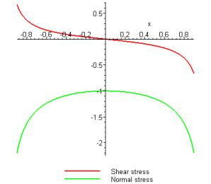
The solution is a bit strange – in addition to the square root singularity at the edge of the flat indenter, we see that the stresses oscillate with increasing frequency as .  For realistic values of , however, the oscillatory behavior is confined to an exceedingly small area near the edge of the punch, however, so this behavior has little physical significance.  For the special case  the oscillatory behavior disappears, and the shear stress is zero.

 

 

 

 

 

Frictionless punch

 

The boundary conditions on the complex potentials for a frictionless punch are

on , while

for large . 

 

Writing out the second boundary condition in full shows that

By the continuation theorem, therefore,  is analytic in the whole plane.  Note also that at infinity

Expanding  as a Taylor series, we conclude that

everywhere.  We now turn to the first boundary condition, which is more conveniently expressed as

Using , we may rewrite this as

on L.  This is once again a Hilbert problem, with solution

where

where the integration constant P(z) must once again be determined from boundary conditions at infinity.

 

Flat Punch

 

Applying this to a flat punch which contacts the surface on , we see that f’(t)=0, giving

Boundary conditions at infinity show that  and so

Again, the contact pressure distribution can be found from

Note that the oscillatory singularity is gone, and we see the same root singularity in pressure at the edge of the punch that we found for the corresponding axisymmetric contact problem.

 

 

Parabolic Punch (2D Hertz problem)

 

A cylindrical punch with radius R may be approximated by the parabolic profile .  A complicating feature in this case is that the contact width is unknown.  However, we proceed by assuming that the contact occurs over a strip , with a to be determined.  Then, we find

The integral can be evaluated using contour integration techniques – but actually MAPLE has no trouble with it, giving

where as before  The boundary condition at infinity gives

 

We must now determine the contact width by examining the behavior of the contact pressure and the shape of the deformed surface.  The contact pressure follows as

(The limiting behavior of  and the square root in the expression for  must be calculated using the approach outlined in solving the Hilbert problem in the preceding section). In addition, the slope of the surface can be calculated from

We see that

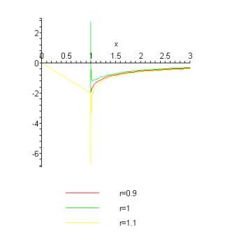
The normalized contact pressure  is plotted for various values of  below. 

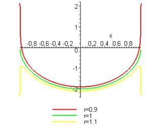
We see that  leads to a tensile stress under the contact – this is inadmissible, since it would cause the two solids to separate.  Similarly, the normalized slope of the surface can be expressed as

The surface slope is plotted below

We find that for  the slope is discontinuous (and singular) at .  The case  is physically admissible, since it corresponds to a separation between indenter and the surface; but  would result in inter-penetration between the indenter and the surface just outside the contact area.

 

Consequently, we conclude that , which gives

 

 

 

 

 

 

 

 

 

 

 

 

 

 

 

 

 

 

 

 

7.8.4 Crack problems

 

In the following, we devise an analogous procedure for solving two-dimensional crack problems. 

 

We assume that the crack occupies some line L on the real axis, and is subjected to a distribution of tractions (not necessarily equal) on its upper and lower surface.  This solution can easily be used to obtain the solution for a crack subjected to far-field loading.

 

As before, our goal is to find an analytic continuation that will simplify the boundary conditions as much as possible.

 

We start with the usual complex variable formulation

Outside the crack the displacements must be continuous across the real axis, which requires that

Following the usual procedure, we express the boundary condition in terms of the functions , which gives

Noting that .  We can therefore re-write the continuity condition as

We therefore conclude that  is continuous on the real axis outside the crack, and is analytic everywhere, and therefore put

where  is a continuous, analytic function. An exactly similar argument applied to the traction continuity condition shows that  is continuous and analytic, and we therefore write

Adding the preceding two equations shows that

We could re-write the governing equations in terms of  and , but in fact it turns out to be more convenient to work with  and .  Eliminating  gives

Any continuous pair of potentials  will automatically satisfy stress and displacement continuity across the real axis.  Unlike the continuation used for half-plane problems, we now have to use two potentials, because we need to find solutions for both the upper and lower half-planes.  We will find that for a symmetric problem  (where upper and lower crack surfaces are subjected to equal and opposite tractions), with vanishing stress at infinity, the potential  vanishes.

 

We now write boundary conditions for the upper and lower crack faces, noting that

so that

Adding and subtracting we see that

giving two Hilbert problems for  and , with general solution

where , and Q(z) and P(z) are arbitrary polynomials, whose coefficients must be determined from conditions at infinity.  Both  and  must be at least  at infinity (if the resultant force applied to the crack surfaces vanishes they must be  ).  This shows that Q(z)=0; and P(z) is at most a constant (if the resultant force applied to the crack surfaces vanishes P(z)=0). 

For the special case where the tractions acting on the crack faces are equal and opposite, we see that , and

For the particular case of a uniform traction  we find that

whence

The stress and displacements can now easily be calculated.  In particular, the stresses on  follow as

The stress intensity factors are defined as

The solution for a crack subjected to remote stress at infinity can be computed by superposing a uniform stress state that induces equal and opposite tractions acting on the crack faces – giving .  One can readily see that the potentials generating this solution are

 

 

 

 

 

 

 

 

 

 

 

 

 

 

 

 

 

Asymptotic crack tip fields for a crack on a bi-material interface

 

The recipe we developed in the preceding section can also be used to solve interface crack problems.  Here’s the scoop.

 

As before, our initial goal is to devise a procedure that will enable us to calculate the fields in both the upper and lower half-plane from a pair of complex potentials, which are chosen so as to reduce the boundary conditions to a Hilbert problem.

 

We follow the usual recipe: (1) Write down the boundary conditions for traction and displacement continuity across the interface in terms of the standard complex variable representation; (2) Express the boundary conditions in terms of the reflected quantities ; (3) Use the result of (2) to identify an appropriate analytic continuation.

 

Since we are trying to solve a bi-material problem, the general complex variable method would require us to find two pairs of analytic functions,  (which are analytic in  ) and  (which are analytic in  ), which generate stresses and displacements in the two regions according to

We now devise an analytic continuation that will automatically satisfy displacement and traction continuity across the real axis.  Displacement continuity requires

while traction continuity gives

We now express these conditions in terms of

As usual, we note that , which enables us to rewrite the boundary conditions as

The second equation can be integrated to get

Both the left and right hand sides of each boundary condition are now analytic functions. The continuation theorem therefore tells us that we can regard each of these combinations of  as a single analytic function, defined in both the upper and lower half-plane, by setting

We can solve for ,  in terms of  and  to see that

Substituting back into the displacement and stress formulas would then give expressions for field quantities in terms of the new potentials.  This is left as an exercise (and in practice it is not really necessary, since we can just determine  whenever we need them).

 

We now require boundary conditions for the new potentials  and  on the crack surfaces.  Since the tractions must vanish, we need to ensure that

Substituting the definitions given above we see that

Note that .  Therefore, subtracting the second equation from the first shows that

This equation is satisfied by  where  is an arbitrary polynomial.  However, boundary conditions at infinity require , and so .  With this substitution, the two boundary conditions reduce to

which is a Hilbert problem

with

The solution to this equation is

where  is an arbitrary polynomial, , and the branch cut for  coincides with the crack.  Again, for vanishing stress at infinity, we require that , where  is some constant. 

 

The stress along the line  ahead of the crack follows as

where .  The asymptotic field is usually expressed in terms of a complex stress intensity factor  such that

which gives

and

The crack opening displacements can also be found

where we note that due to the branch cut

Some algebra reduces the result to