 EN224: Linear Elasticity
Division of Engineering
8.3 Applications of Minimum Potential Energy I: Approximate Solutions.
The principles derived in the preceding section have two important applications. They can be used as a formal framework for devising approximate solutions to boundary value problems in linear elasticity. In addition, they can be used to obtain rigorous bounds on certain properties of solutions to boundary value problems.
We will show how one can use energy methods obtain approximate solutions to boundary value problems by looking at two examples. In each case, the approach is to assume that the displacement field can be described using a reduced set of field variables, and then to find the solution within this class that minimizes the potential energy. This does not guarantee that the approximation will be accurate – that depends on whether the assumptions were reasonable. It does guarantee that you found the best possible solution within your approximation.
Euler Beam Theory
We will re-derive a theory that should be familiar to you, from our new perspective.
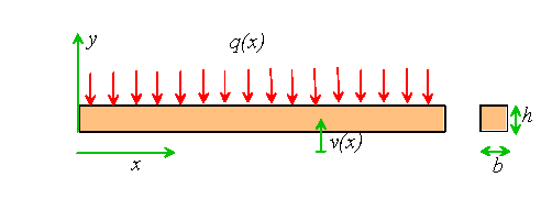
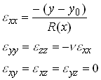
Consider a slender rod with rectangular cross section, subjected to
uniform pressure q(x) on its top surface. Assume that the rod is
an isotropic, linear elastic solid with Young’s modulus E and
Poisson’s ratio![]()
The boundary conditions at the ends of the bar will be left unspecified for the time being.
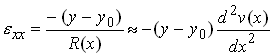
We proceed by approximating the displacement field within the bar. We will suppose that the strains at any given cross section are completely characterized by the local curvature of the beam, so that at a given cross section x
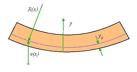
Here,![]() is the height of a fiber in the beam whose length is
unchanged.
is the height of a fiber in the beam whose length is
unchanged. ![]() must be determined as part of the solution.
must be determined as part of the solution.
The displacement and strain fields are therefore completely characterized
by![]() and R(x). Rather than solve for R, we will
approximate the curvature at x by the second derivative of the vertical
deflection v, so that
and R(x). Rather than solve for R, we will
approximate the curvature at x by the second derivative of the vertical
deflection v, so that
Now, we want to find v(x) and![]() that will best approximate
the actual displacement field within the bar. We will do this by choosing
v and
that will best approximate
the actual displacement field within the bar. We will do this by choosing
v and ![]() so as to minimize the potential energy of the solid.
so as to minimize the potential energy of the solid.
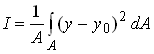
Begin by computing the potential energy. It is straightforward to show that the strain energy density is
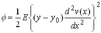
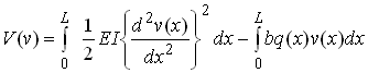
Hence
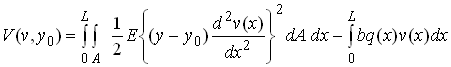
Here, we have neglected the small additional deflection of the beam
surface due to![]()
We now wish to minimize V with respect to v and![]() . Do the latter first:
. Do the latter first:
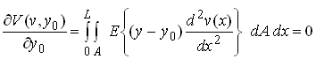
which is evidently satisfied for any v by choosing
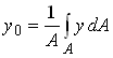
We can simplify our expression for potential energy by defining
so that
Now turn to the more difficult problem of finding v that will minimise V. Note that if V is a minimum it is also stationary, which implies that
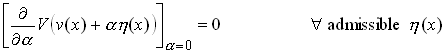
Here, `admissible’ means that![]() must satisfy any constraints
on v or its derivatives. We will return to this issue later, when
we finally specify boundary conditions on the beam.
must satisfy any constraints
on v or its derivatives. We will return to this issue later, when
we finally specify boundary conditions on the beam.
This is another way of saying that any change in v causes no change in V to first order.
Using this condition, we see that
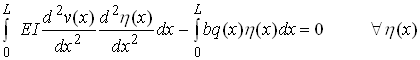
We are none the wiser as a result of this exercise, but if we integrate the first integral by parts twice, we find that
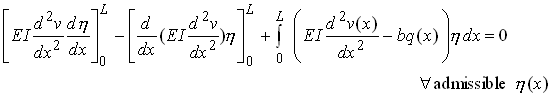
Hence, we must satisfy
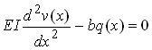
to ensure that the third term in this expression vanishes. This gives us the required governing equation for v. However, we still need to deal with the first two boundary terms.
There are several ways to prescribe boundary conditions on the ends of the beam to ensure that V is stationary.
We may prescribe v and/or its first derivative at one or both
ends. If v is prescribed, we must ensure that![]() , so as not
to violate the boundary condition. In this case, the second boundary term
is automatically satisfied. If there are no constraints on v, then
we must set
, so as not
to violate the boundary condition. In this case, the second boundary term
is automatically satisfied. If there are no constraints on v, then
we must set
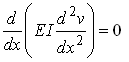
to ensure that V is stationary. We know from elementary strength of materials courses that this is equivalent to the condition that the shear force vanish on the end of the beam.
Similarly, if dv/dx is prescribed, then we must ensure that ![]() .
The first boundary term then vanishes. If there is no constraint on dv/dx,
then we must set
.
The first boundary term then vanishes. If there is no constraint on dv/dx,
then we must set

This is equivalent to setting the bending moment to zero at the end of the beam.
Clearly, one could extend this procedure to account for tractions acting on the ends of the beam. The details are left as an exercise. A nice feature of the variational approach that we followed here is that the appropriate boundary conditions follow naturally from the variational principle (indeed, the boundary conditions are called `natural’ boundary conditions). This turns out to be particularly helpful in setting up approximate theories of plates and shells, where the boundary conditions can be very difficult to determine consistently using any other procedure.