 EN224: Linear
Elasticity
EN224: Linear
Elasticity 
Division of Engineering
4. 2D Static Boundary Value Problems I: Saint-Venant Torsion
So far, we have been trying to solve fully 3D (or axisymmetric) boundary value problems. There are very few 3D problems that can be solved exactly. Instead, we normally approximate the problem somehow, to try to reduce it to two dimensions.
For the remainder of this course, we will discuss various 2D approximations to boundary value problems, and we will consider some techniques that can be used to solve them.
4.1 General Saint-Venant Problems
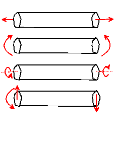
Saint-Venant devised a procedure for obtaining approximate solutions to long, slender bodies, which are subjected to end loading. The solutions were of great practical significance, since they provided a way to design structural members.
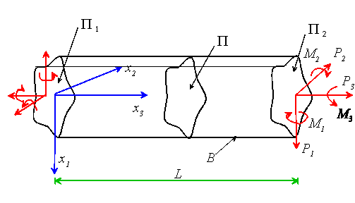
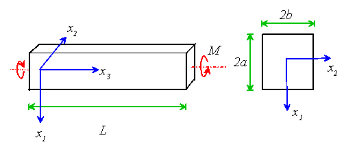
Consider a slender, cylindrical rod, whose length L greatly exceeds
any cross-sectional dimension. Assume that the lateral boundary of the
rod B is free of traction. The ends of the rod![]() and
and![]() are subjected to a distribution of traction, chosen so as to guarantee
overall equilibrium of the rod (i.e. resultant forces and moments on the
two ends are equal and opposite.) We will not specify the distribution
of traction on the ends of the rod in any detail: instead, we prescribe
the resultant force and moment on the ends, and then try to find
any solution, which satisfies the weak boundary conditions. The
solution is not unique, but Saint-Venant’s principle guarantees that
all the solutions will approach one another away from the ends of the rod.
are subjected to a distribution of traction, chosen so as to guarantee
overall equilibrium of the rod (i.e. resultant forces and moments on the
two ends are equal and opposite.) We will not specify the distribution
of traction on the ends of the rod in any detail: instead, we prescribe
the resultant force and moment on the ends, and then try to find
any solution, which satisfies the weak boundary conditions. The
solution is not unique, but Saint-Venant’s principle guarantees that
all the solutions will approach one another away from the ends of the rod.
To make this precise, we seek![]() . with
. with
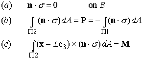
It is convenient to express these boundary conditions in terms of stresses in the rod:
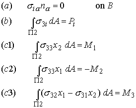
There are four general classes of Saint-Venant problem corresponding to various choices of end loading.
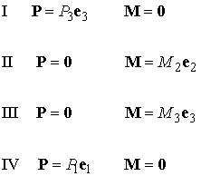
Cases I and II are solved in elementary strength of materials courses. We will investigate case III here. You have probably seen a simplified version of case IV in strength of materials courses: the general treatment is complex and will not be discussed here. If you are interested, you can find a nice discussion in Sokolnikov’s book (see TEXTS).
4.2 Solving Torsion problems using warping functions
You probably recall the solution for torsion of a circular shaft from
your youth. If the shaft is circular, symmetry considerations lead us to
the conclusion that each cross section![]() must remain planar. We
then assume that the left hand end of the shaft
must remain planar. We
then assume that the left hand end of the shaft![]() is held fixed,
while the right hand section
is held fixed,
while the right hand section ![]() is rotated through some (small)
angle
is rotated through some (small)
angle ![]() about the
about the ![]() axis.
axis.
Since all cross sections remain planar, the only thing that a particular
cross section can do is to shear or stretch in its own plane (impossible
by symmetry and the boundary conditions on the r=a), or rotate about
the![]() axis. Symmetry considerations finally lead us to the conclusion
that the rotation must vary linearly along the length of the shaft.
axis. Symmetry considerations finally lead us to the conclusion
that the rotation must vary linearly along the length of the shaft.
Thus, the displacement field in a circular shaft has the form:
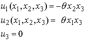
Here![]() is the twist per unit length of the shaft.
is the twist per unit length of the shaft.
The stress field may readily be deduced, and resultant torque acting on the ends of the shaft may be computed from the result.
Solution for general cross sections
We use the solution for a circular shaft as the starting point for our more general solution.
The lateral boundary conditions still suggest that in-plane stretching and shearing is not likely to take place (we can only really be confident that this is the case if we know how to solve plane problems in elasticity, but that’s a story for a future class). However, there is no longer any reason to suppose that plane sections will remain plane. Since all cross sections have the same shape, it is natural to suppose that they will all deform the same way, so we suppose that the displacement field has the form
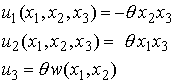
Here, w is known as the warping function, and needs to be determined. We need field equations and boundary conditions for w, as well as a way to determine the twist.
The state of strain in the rod follows as
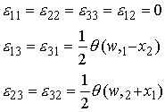
and the stresses are
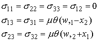
Equilibrium requires
This is the governing equation for w that we were looking for.
Next, check out the boundary conditions. We need to satisfy the traction free condition on B, as well as the weak boundary conditions on the ends of the rod. Let us check the boundary conditions on B first. Consider a general cross section, as shown:
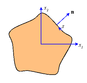
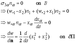
where we have noted that
Thus, the normal derivative of w is prescribed on the boundary, and is determined by the shape of the cross section.
Next, check the resultant forces acting on the cross section. We need all the resultant forces and moments except the twisting moment to vanish. First, check the transverse forces acting on the ends of the rod:
In addition, the boundary conditions involving![]() are clearly
satisfied, since
are clearly
satisfied, since![]()
The only remaining boundary condition is the one involving the twisting moment:
Hence, to satisfy the final boundary condition we must choose

where
The first term in the expression for k is evidently the polar moment of area of the cross section. The second term corrects the solution for the effects of warping.
We can find another expression for the warping term that shows clearly that warping always reduces the stiffness of the shaft:
Now recall that
(this is one of the boundary conditions on w), so that
where we have used the fact that w is harmonic. Hence, our alternative expression for k is
showing clearly that the warping reduces the stiffness.
One final point: notice that we never said where the origin for our coordinate system is! It turns out to make no difference. It is left as an exercise to show this.
Example using the Warping function
We will attempt to compute the warping function for a shaft with rectangular cross section, and use the result to deduce the torsional stiffness of the shaft.
We seek a warping function w that satisfies
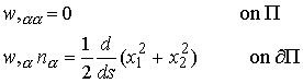
For the rectangular cross section, the boundary conditions reduce to
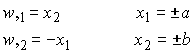
We can simplify the boundary conditions slightly by setting![]() and
solving for v rather than w. Clearly, v must be harmonic,
and must satisfy
and
solving for v rather than w. Clearly, v must be harmonic,
and must satisfy
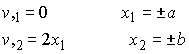
The first boundary condition is now independent of x, which is helpful.
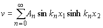
A solution of ![]() which has the necessary symmetries is
which has the necessary symmetries is
To satisfy ![]() on
on ![]() we must set
we must set![]() , which requires
, which requires
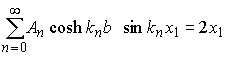
We may the choose the coefficients![]() to satisfy the remaining
boundary condition
to satisfy the remaining
boundary condition![]() on
on ![]() . Clearly, we must satisfy
. Clearly, we must satisfy
This may easily be solved for![]() by taking the finite sin transform
of both sides:
by taking the finite sin transform
of both sides:
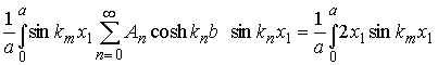
which yields
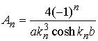
So, we finally conclude that a suitable warping function for our problem is
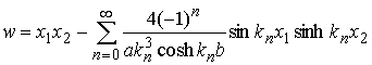
with
The stiffness of the shaft follows as
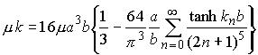
Although all our results remain in the form of infinite series, one finds that the series converge very quickly and evaluating a few terms is usually sufficient. For the particular case of a square shaft, one finds
4.3 Solving Torsion problems using Prandtl stress functions
When solving 3D problems, we found it convenient to solve for displacement components. We followed the same approach to develop the warping function for torsion. For plane problems, we can often devise another approach: instead of trying to solve for displacements, we can attempt to solve for stresses. We normally try to find a way of representing stress fields in terms of scalar potentials, chosen so as to satisfy automatically the equations of equilibrium. The compatibility equations provide governing equations for the relevant potentials.
We will develop a similar approach for torsion problems. In this case, it is most convenient to start with the warping function representation outlined in the preceding section.
Recall that the warping function w satisfies

![]() Since w is a harmonic function, it has a conjugate
Since w is a harmonic function, it has a conjugate![]() , which is related to w through
, which is related to w through

Evidently![]() is harmonic. Given w, we can always find
is harmonic. Given w, we can always find![]() (at least to within an arbitrary constant) and vice-versa. We note in passing
that
(at least to within an arbitrary constant) and vice-versa. We note in passing
that
is an analytic function: the relationship of w to ![]() are the Cauchy-Riemann
conditions.
are the Cauchy-Riemann
conditions.
If we choose to solve for![]() rather than w, our boundary
conditions are
rather than w, our boundary
conditions are
and recalling that
we find
so we may choose
since we only require![]() to within an arbitrary constant.
to within an arbitrary constant.
We can simplify this boundary conditions by introducing a new potential, known as the Prandtl stress function
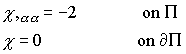
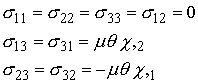
Evidently, the governing equations and boundary conditions on![]() are
are
Using the expressions for the stress components in terms of w
given in the preceding section, together with the definition of ![]() ,
we find that the stress components may be computed as follows
,
we find that the stress components may be computed as follows
This shows the advantage of using the stress function approach. The
expressions for stress fields are simpler than those in terms of the warping
function, and the boundary conditions on ![]() are considerably nicer
than those on w. The cost is a slightly more complex governing equation
for
are considerably nicer
than those on w. The cost is a slightly more complex governing equation
for![]() .
.
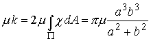
Finally, the torsional stiffness is![]() , where k is
, where k is
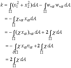
where we have used the boundary conditions to obtain the last line.
Example using Prandtl’s stress function
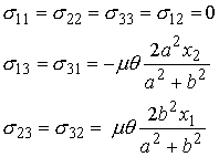
Consider a shaft with an elliptical cross section, which occupies the region
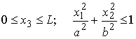
Suppose that the shaft is subjected to a twisting moment M. Find the state of stress in the shaft, and its torsional stiffness.
We will solve this problem using Prandtl’s stress function. We need to find a function that satisfies
Consider the function
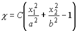
This clearly satisfies the boundary condition. To satisfy the field equation we must choose

The state of stress in the shaft then follows as
Finally, the torsional stiffness is given by