Assgn 6: Periodic Waveforms, Sample Rate Aliasing, Fast Fourier Transform & Digital Filtering
(to be done solo)

Background:  The sampling theorem will be one of the most important constraints you'll learn to work with in instrumentation. The sampling theorem says if the maximum frequency in the analog input signal is less than half the sampling rate, you can achieve "perfect reconstruction" of the input waveform on the digital side. If the max input freq > sampling rate then aliasing of high frequencies will occur; the aliased frequency is determined from a "mirror image" formula; an aliased high frequency is a form of noise.

In this lab you will observe aliased frequencies. As a prelude, you will learn more about waveform generation, given our need for periodic signals. Then you will use the Fast Fourier Transform (FFT) in the 54622A digital 'scope and in LabVIEW's "Power Spectrum" to demonstrate aliasing in various circumstances.

Requirements: See the 7 challenges below. For the sake of efficiency, let's say you're prepared to finish show us something from all 7 challenges within 30 minutes or less. If you need help, fine, but if the helping takes more than 30 minutes, go off and reread the documentation and come back the next day...

(1) The 33120A Waveform Generator: Each setup has the 300-page Users Guide for your study. For this lab we will care only about the first 3 chapters of the Guide. When asked, you should be able to display any of the 11 waveforms listed at the top of page 298 (OK, "DC volts" isn't really a waveform, but you may show it to us anyway, -see page 24- and realize you have a source of DC signal other than your triple output power supply). See page 175 for diagrams of the "built-in arbitrary waveforms". Why do they call one of the waveforms Cardiac?

(2) For each of the 9 periodic waveforms you should be able to change frequency, amplitude and offset. For pulses, you should understand what Duty Cycle is and show us pulses of 20% to 80% duty cycle. For any of the parameter changes you should be able to use the knob, or enter numbers. (See Chpt 1 of the Guide).

You should be able to tell us what's on the SYNC output, on the 33120A front panel. Or show us on the scope! Why is it called "SYNC"?

Become familiar with the Menus of the 33120A.
(3a) See Chpt 2 of the 33120A documentation. Be able to navigate to Menu D and change from 50 Ohm to High Z for the output impedance. Show how the amplitude reading of a waveform changes when you go from 50 ohm to High Z.

(3b) Create on the 'scope, from the 33120A, a 9 cycle burst of square wave pulses at 40KHz. Have the burst triggered by the approx 1KHz rising edge from the 54622A scope probe test output. Ext Trig is an INPUT on back of 33120A. Note that on p100 of the Users Guide it states that pressing the SINGLE button enables EXT TRIG. On the 33120A Menu system or otherwise you would like to have the burst rate much lower than 40KHz, say 400 Hz. The menu system under Menu A, items 4, 5, 6, 7, covers relevant burst parameters, including rate and count.

(3c) Be able to use Menu B to demonstrate a logarithmic sweep of frequencies. Can you trigger a single sweep? See p. 98 of the 33120A Guide.

(3d) From the waveform generator to the Digital Multimeter AC volts input arrange that a 1000 Hz sinewave has the same RMS amplitude (1.00) on both instruments.

(4) Sinewave purity.
Use your Agilent 33120A waveform generator to set up a 2v p-p sinewave, at 8KHz, and send it on a BNC cable to channel 1 of the 54622A scope. Press the Math button and highlight the FFT feature. Rotate the time base knob until the sample rate is 40KHz. Look at the resulting spectrum. Is there a peak at 8KHz? How broad is the peak? Are there any harmonics? (freq's at multiples of the fundamental--in this case 8KHz). For a cleaner display, suppress the time base view of the channel 1 signal. Switch to pulse, triangle or sawtooth waveforms to see more prominent harmonics.

Is the amplitude scale on the 54622A spectrum log or linear?

(5) Aliasing. Move the sinewave frequency around, 1000 Hz at a click. Does the spectrum peak shift as you would expect?
Increase the frequency to 19, 20KHz, then to 21 KHz. At what frequency is 21KHz aliased? Why is 21KHz aliased? To answer, Recall the Sampling Theorem and be able to say something about your sample rate... Increase the input frequency up to 39KHz. What is the aliased frequency? What about the alias of 42KHz?

(6) Now try a square wave at lower frequency, like 6KHz. Increase the fundamental frequency. In the spectrum, can you make an alias of the first harmonic add with (be equal to...) the fundamental?

(7) Spectrum Analysis in LabVIEW. Send your 8KHz sinewave into an analog input on the green connector card. Acquire 1 second of the waveform using the AI Acquire Waveform subVI, setting the sample rate at 40KHz. Use the Power Spectrum subVI from the Analyze:Signal Processing:Frequency Domain Function Menu. Display the spectrum with a GRAPH, NOT CHART waveform. Do you see the same spectrum in LabVIEW that you saw on the digital scope? Be aware that the amplitude of the spectrum peak may be much less than 1.00!

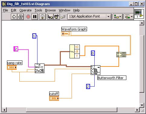
(7B) Now that you can sample correctly, lower your sample rate to 400 Hz and send the sample rate also to the sample number input(1 second of sampling). Send the output of the waveform acquisition to a LP 2nd order Butterworth filter with a cutoff of 10Hz. Send the output of the DAQ icon and the Butterworth filter to one Waveform graph. Lower the frequency of the waveform generator to 6, 10, 14 Hz and show filter input vs output. See suggestions below, for showing the unfiltered and filtered waveforms on the same plot.


Possible FTQ: Where will be the spectrum peak for a sinewave at a certain frequency above the Nyquist rate? What's a formula for the frequency where the fundamental is exactly equal to the alias of its first harmonic?

Further Reading: Lectures notes on aliasing from the EN123 archive website. You might also try typing "Alias Frequency" into google and see what happens.