Lab
8T: Using the Thor DRV001 micro-advance to flex (repeatably) individual blaberus
exoskeleton spines
(2011: Kelsey MacMillan [KJM] UTRA project)
Background:
We assume here you have finished Lab 8. In this more quantitative look
at blaberus spines you will use a precise Thor linear actuator (DRV001) to probe
a individual spines for their response to angular deflection (and rate of deflection,
and direction). Two linked LabVIEW programs, running simultaneously, will be
used to control the probe and collect spike response data. All data will be
saved to MATLAB data files (.mat) and then analyzed in MATLAB itself, rather
than in a MATLAB script running in LabVIEW.
Blaberus and the probe will be set up and viewed with an AO dissecting microscope.
The microscope is additionally compatible with a microscope camera which can
be used to capture a video of the spine deflection that occurs as a result of
the probe advancing.
What follows: Details of the hardware and software you will need in Lab 8T.
Hardware:
ThorLabs DVR001 ($700) Motorized Linear Actuator
(See detailed product information at: http://www.thorlabs.com/NewGroupPage9.cfm?ObjectGroup_ID=1881)
This device, a motorized linear actuator, is capable of linear travel with a
repeatable precision of < 1 micron. The motorized actuator has been fitted
with a split-tip probe, which allows for precise contact with a single spine.
Controls for the actuator occur through a ThorLabs BSC101 controller ($1300)
which receives instructions from the main computer. ThorLabs produces associated
software for the controller with a simplistic GUI. In our case, however, a LabVIEW
program has been written to allow specialized control of the actuator for the
purposes of data collection.
Mechanical Cradle
Because the linear actuator has only 8mm of total travel, an adjustable arm
has been built (KJM) to hold the actuator/probe in place at an appropriate distance
from the specimen. The cradle can be moved vertically by adjusting the height
of the supporting lab jack. It can also be moved around two axes of rotation,
one at the "elbow" gear junction, using a mechanical pin brake, and
the other at the "wrist" junction, by shifting the position of actuator/probe
in the vise grip.
[Images needed]
Specimen Platform
The leg preparation is to be placed on a copper platform, which also functions
as a ground. The copper has been machined out and filled with a transparent
silastic compound which may be penetrated by dissecting needles placed through
the cockroach leg. By loosening the knob at the side of the platform, it is
possible to adjusting the angle of the platform.
Electrodes:
Paul Waltz has designed and fabricated an electrode holder that positions
3 needle electrodes 2.5 mm apart to penetrate the silastic and hold the preparation
in place.
Microscope Camera
The OptixCam camera can be inserted in the right eye piece of the dissecting
microscope, and connected to the main computer via USB port. Image and video
capture occurs in the OCView associated software, which can be found in the
Start menu list of programs.
Software in IP folder...
LabVIEW VI (A): 8T_11_ThorController.vi
LabVIEW virtual instrument (VI) sends commands (either sequenced or instantaneous)
to the THORLABS BSC101 controller for the DVR001 linear actuator. All controls
are accomplished by ActiveX controls which appear as "Invoke Nodes"
in LabVIEW. Each ActiveX Invoke Node takes user inputs in the form of numerical
codes and then either "gets" properties from the Thor controller or
"sets" properties of the controller, i.e. sends instructions to the
linear actuator. For specific information on the function of each Invoke Node,
right click the node and consult the Help menu.
Using the VI it is possible to specify the positions of any number of absolute
moves, along with the maximum velocity the actuator probe should travel at,
and the time the device should wait to initiate the next move. While moves are
being completed according to sequencer parameters, the VI program queries the
BSC101 controller for its current position several times per second, so as to
track the position of the actuator in real time. An array of positions and their
corresponding times are saved in a .mat-file over the course of each program
execution. These arrays are loaded as variables in the MATLAB program complimentary
to this VI.
Trigger functionality of the BSC101 controller is also accessed by the LabVIEW
VI. During the second phase of the program, the VI instructs the controller
to output a logic HIGH from its trigger I/O pin at the moment when the actuator
begins to execute a sequenced move. This logic HIGH can be read by another device
or VI to set off simultaneous program execution.
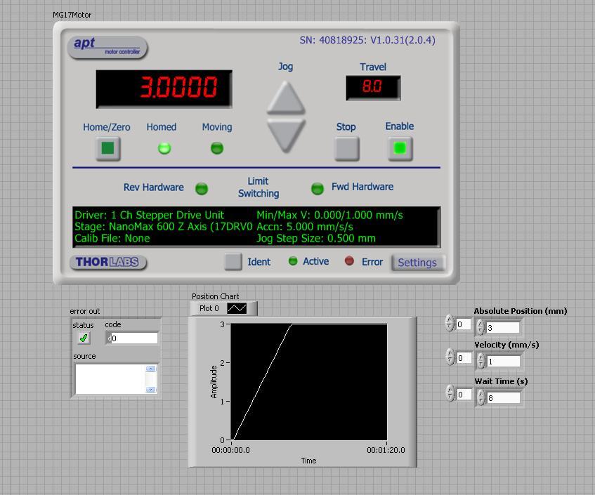
Below is an image of the front panel of the fully functional VI. The arrays
at the bottom right of the front panel are controls used to input position and
velocity directions to the Thor controller. The Thor panel at the top center
of the front panel can be used to give instantaneous instructions to the Thor
controller, and so check functionality.
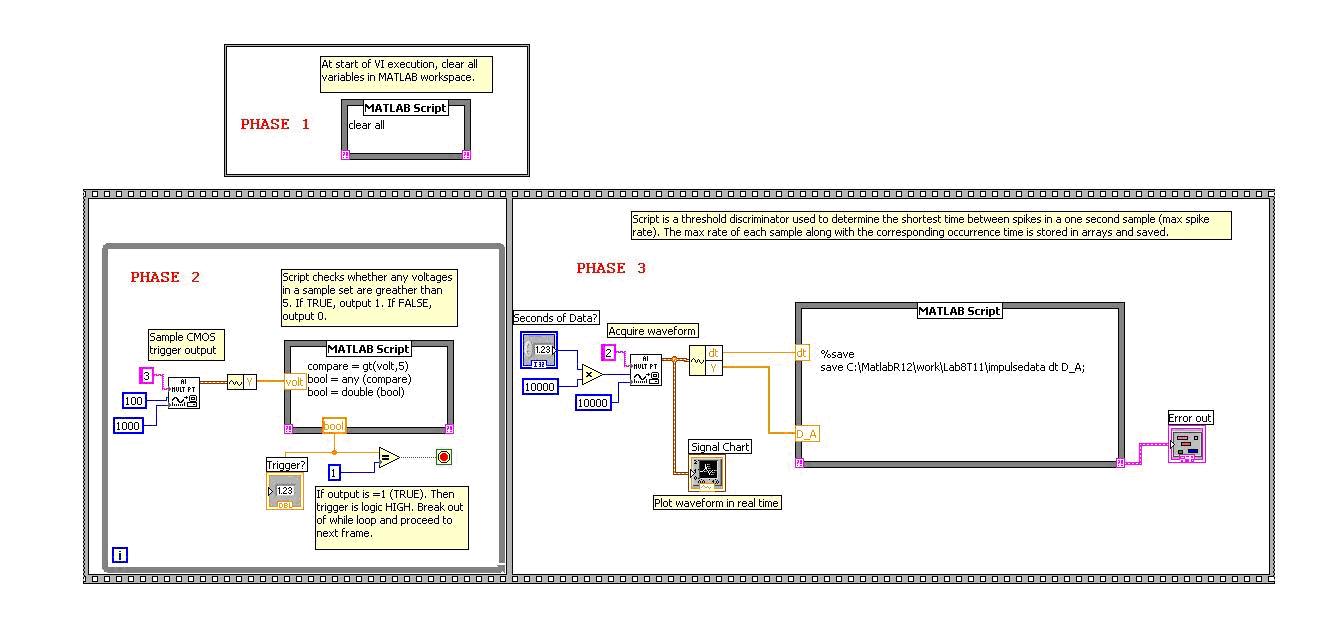
LabVIEW VI (B): 8T_11_PulseRate.vi
This VI (block diagram shows below) is similar to the one used in Lab 8. This
VI differs because it collects data over an extended period of time, then saves
all data to a *.mat file, which can be loaded in a MATLAB m-file. All data analysis
is performed in a MATLAB m-file, rather than in a MATLAB script in the VI. Also
different: the VI, once started, waits in a while loop until it detects a logic
HIGH from the NI board, at which point it breaks out of the loop and proceeds
to collect electrical impulse data. The logic HIGH should originate from the
8T_11_ThorController VI, and indicate that the actuator probe has begun moving.
The period of time over which electrical data is collected is specified by a
control in the VI front panel.
 MATLAB
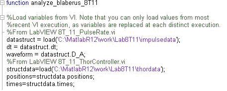
M-File A: analyze_blaberus_8T11.m
MATLAB
M-File A: analyze_blaberus_8T11.m
All data collected from both VI's is loaded then analyzed in this matlab
script. The code for loading saved .mat files is included below. Specifically,
the data consists of position data for the linear actuator, and electrical impulse
data from the electrodes at the specimen. The rest of code in this file (not
shown) plots both data sets and then uses a threshold discriminator to count
spikes.
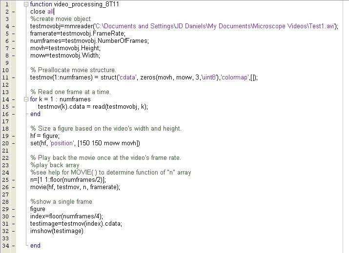
MATLAB M-File B: video_processing_8T11.m
MATLAB's image processing tool box allows images and video to be loaded,
manipulated, analyzed, and played back. This m-file, in the image below, uses
just the basic image processing tools. It loads the file, the plays it back,
and then selects a single frame to display as an image.
Requirements:
Your goal is to assemble
a VI + Thor controller to move the probe next to a spine while collecting spike
data. The data will be saved for analysis. This will require that you take these
steps to get all phases...in phase...
1. Place the specimen
on the platform and connect electrodes to amplification system and NI input
board.
2. Move the motor with probe into the mechanical cradle; adjustment position
of the probe tip with aid of dissecting microscope.
3. Plug in all necessary wires for amplifier and sound system; start the Thor
BSC101 controller, and open both LAB8T_11 VI's.
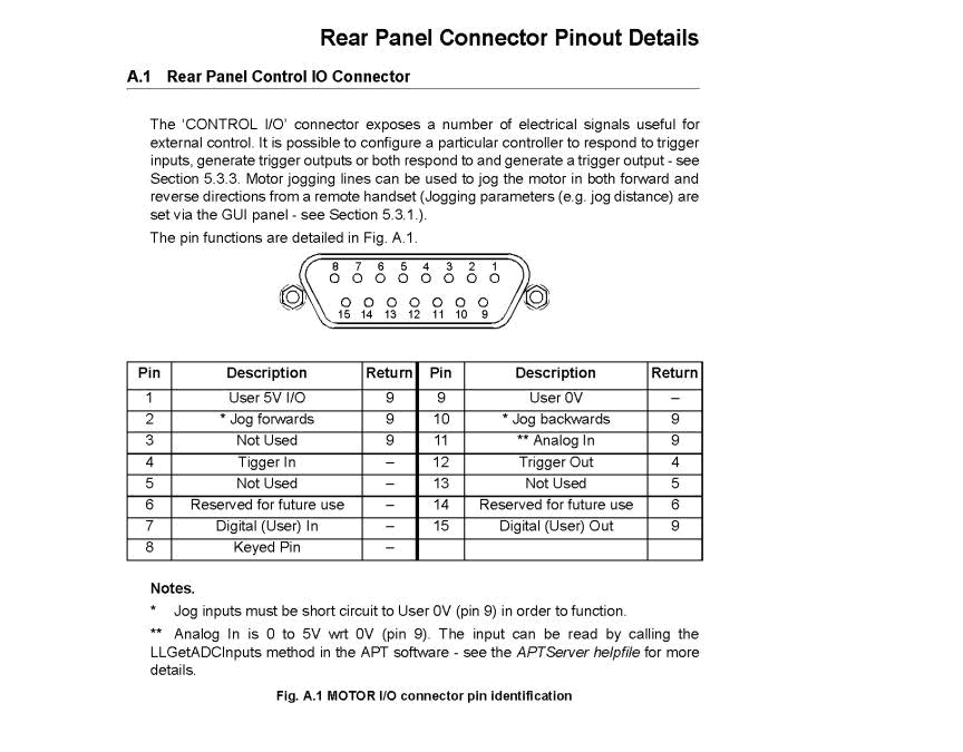
4. Hook-up the trigger, from the Thor controller "Control IO" pins
to the NI input board. You will need to consult the following pin diagram to
determine which pin to wire to the NI board. Remember to include a reference
ground pin wire.
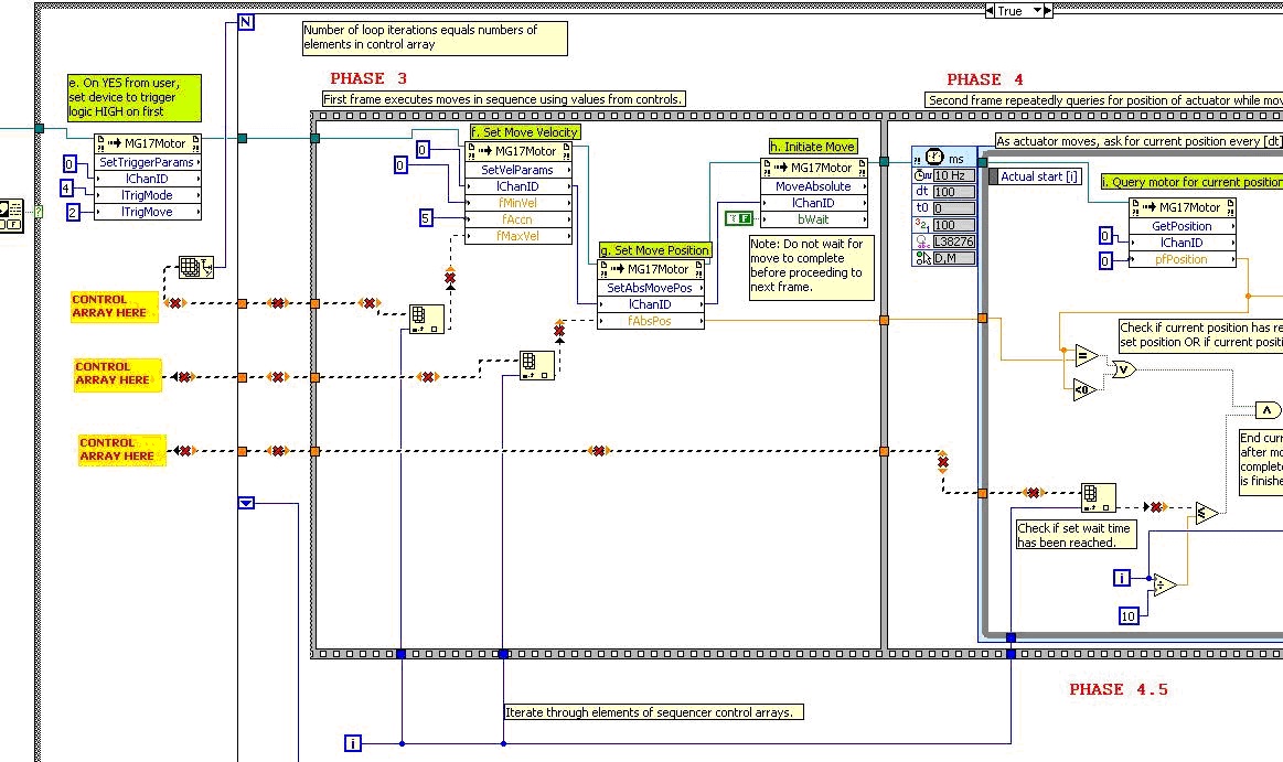
5. Build the VI shown
below. Start with the broken default Lab_8T11_ThorController.vi in the IP folder.
Add the control arrays. Use the arrays to program the probe to move to a pre-selected
absolute position, hold the position for a set amount of time, then return to
home. You will have to figure out the basics of how the VI is working to do
this. To help you out, we've placed red and yellow signs that indicate where
to place the missing arrays controls.
6. Check that the probe
is moving as you want it to, both by running the Thor Controller VI and by playing
with the controls on the front panel. You can observe the movement of the probe
and spine under the dissecting microscope.
7. To run the experiment, first start the 8T_11_PulseRate VI, which will wait
in the while loop. Then run the 8T_11_ThorController VI. On user input "YES",
the Thor controller should trigger and the other VI should start collecting
pulse data. These two VI's running simultaneously will allow electrode data
to be collected while the probe is moving as programmed, thereby allowing detailed
response analysis. Use the charts in either front panel to check in real time
that the experiment is proceeding.
8. Now pull up the
analyze_blaberus_8T11 m-file in MATLAB. Run the m-file to check data by plotting.
9. In the m-file you
must alter the threshold discriminator to make it a window discriminator, just
as you have done in previous labs.
Follow-Up Questions:
1. Using the data collected, relating probe position to afferent response,
develop a model relating the position and velocity components of the probe motion
to the frequency response from the stimulated spine.
2. Additionally, by applying analytic geometry, determine how the linear motion
of the actuator translates to the deflection of the spine.
4-point bonus:
Make a video of spine deflection due to probe movement!
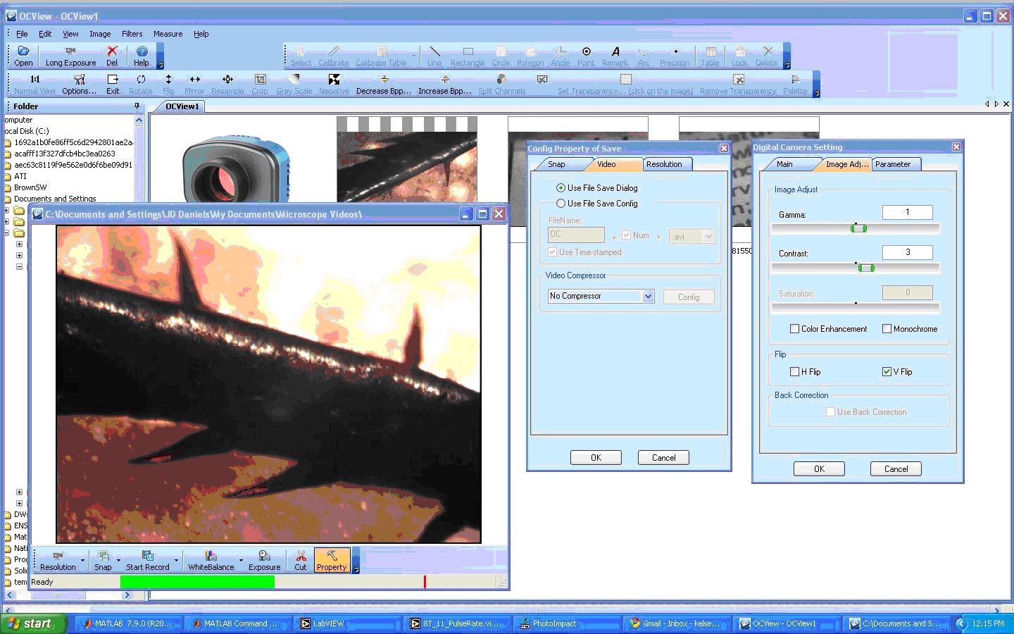
Try setting up the microscope video camera: First line up the dissecting microscope
over the probe and specimen, then replace the right eye piece with the microscope
camera lens. Plug the camera into the main computer and start the OCView software.
Use the OCView software to help you adjust the dissecting microscope and bring
the image on screen into focus. To illustrate, I've included a screenshot of
the camera and software in action.
Because MATLAB image processing is limited by the computer's available RAM,
you should take videos at the lowest resolution possible. Configure the video
capture properties and select the lowest resolution.
Start the camera capture, saving the AVI file to the directory of your choice.
Remark only, that this must be the same directory from which the video file
is loaded in the complementary MATLAB m-file. Next, restart the T_11_PulseRate
VI, followed by the 8T_11_ThorController VI. This allows you to collect probe
position data, impulse response data, and image data simultaneously.
After re-running the experiment, stop the camera. Open video_processing_8T11.m
in MATLAB. This will allow you to play back the video you've just captured.
Super 3 point bonus:
Modify the video_processing_8T11.m code, so that the MATLAB file only plays
back the frames that capture the experiment in action, not the dead space on
either end.
HINT: To do this you will have to change the inputs to the MOVIE ( ) function.
Consult the MATLAB help menu for the function "MOVIE" to determine
how to make the edit.