Necker Lab
(2014--Aneesh Heintz, Anjaney Shrivastav)

Background: The Necker cube is an optical illusion first published as a rhomboid in 1832 by Swiss crystallographer Louis Albert Necker. When staring at one corner of the cube, two different orientations of the cube can be seen.

See Necker Cube on the internet at wisebytes.net

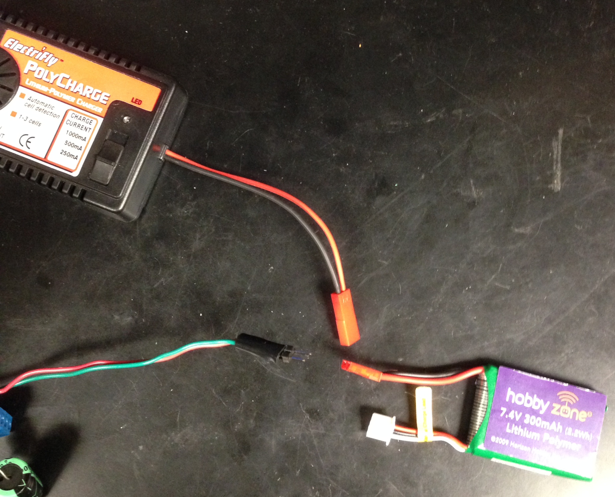
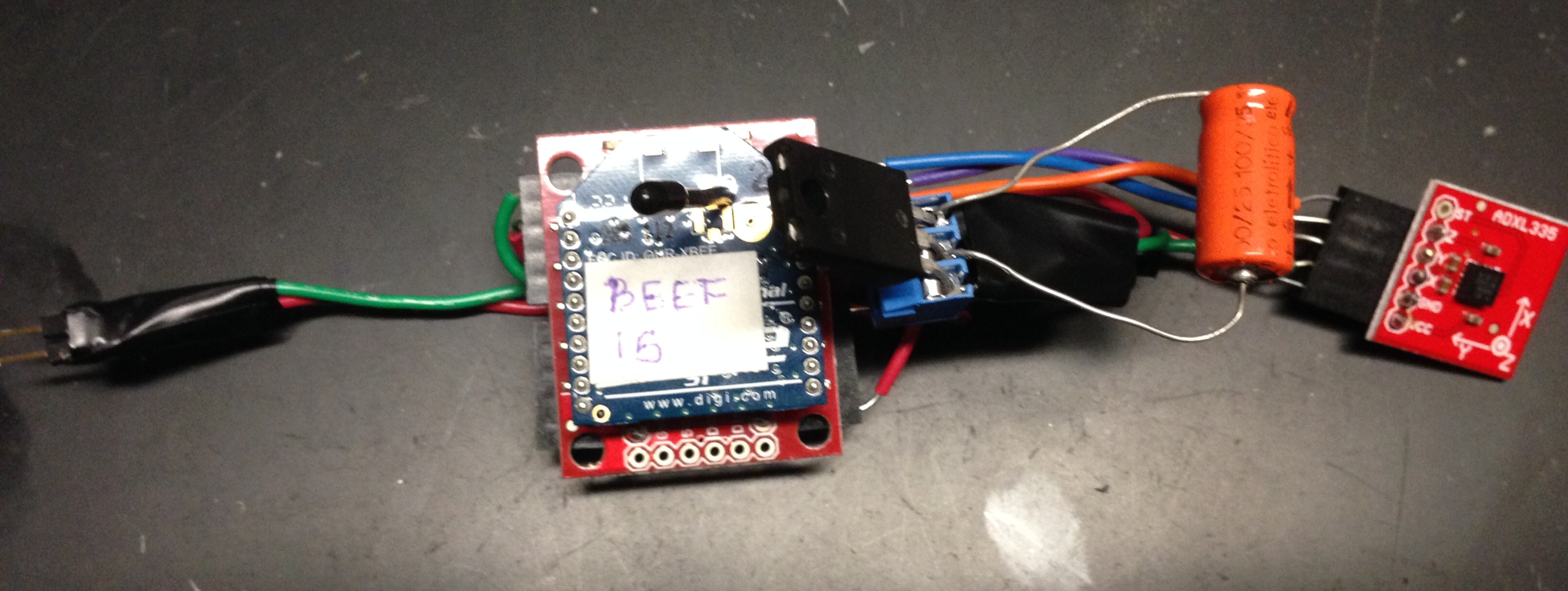
Battery Connection:

After the battery (bottom right) is removed from the charger (top left) and connect it to the transmitter (bottom left).

You should verify that a red LED located on the XBee receiver is on, indicating that the transmitter is currently transmitting data. As soon as the transmitter receives
power it will begin to transmit data

.

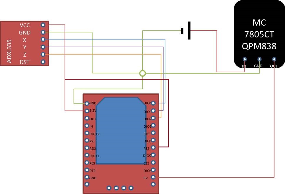
Schematic of Circuit:

.

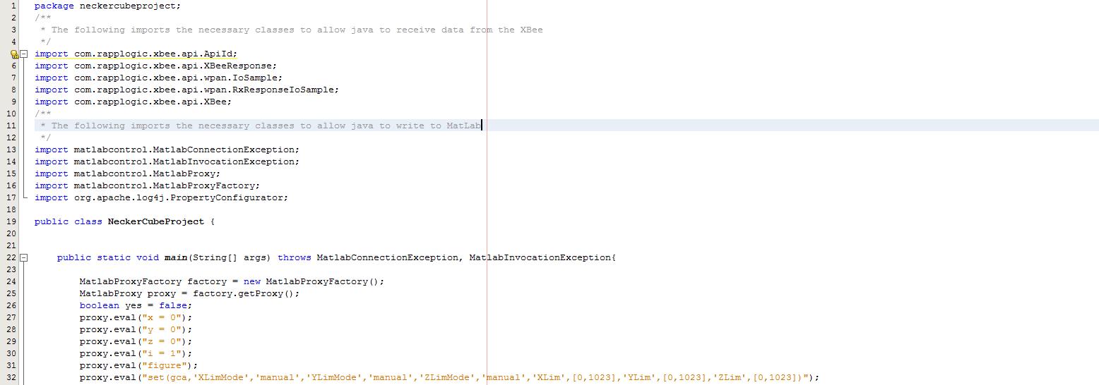
Code: Java Code running in Matlab:

The following imports the necessary classes to allow Java to receive data from the XBee.

import com.rapplogic.xbee.api.ApiId;
import com.rapplogic.xbee.api.XBeeResponse;
import com.rapplogic.xbee.api.wpan.IoSample;
import com.rapplogic.xbee.api.wpan.RxResponseIoSample;
import com.rapplogic.xbee.api.XBee;

The following imports the necessary classes to allow Java to receive data from the XBee.

import matlabcontrol.MatlabConnectionException;
import matlabcontrol.MatlabInvocationException;
import matlabcontrol.MatlabProxy;
import matlabcontrol.MatlabProxyFactory;
import org.apache.log4j.PropertyConfigurator;

These classes are located in the folder "NeckerCubeLab".

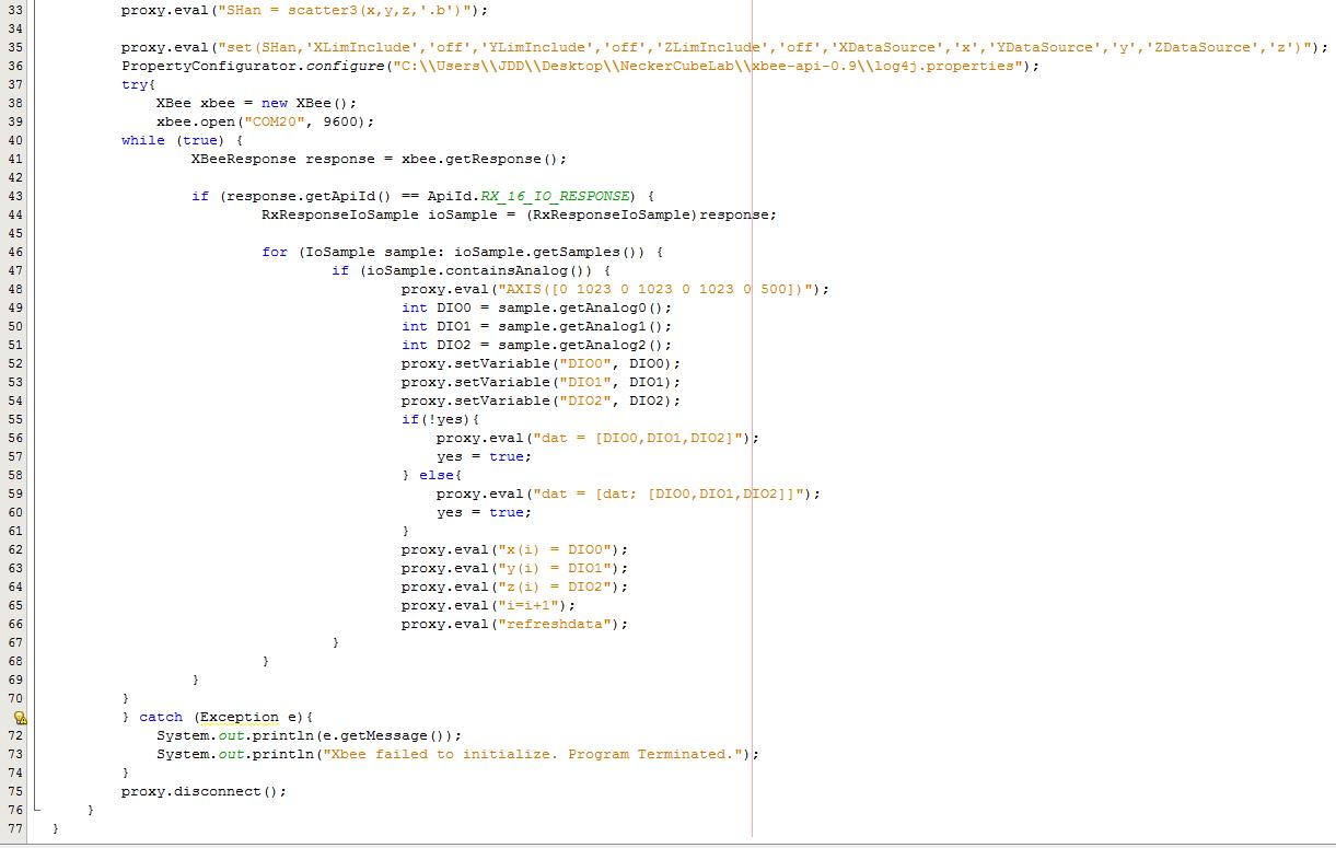
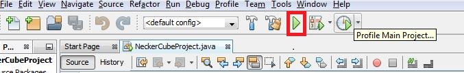
In order to edit or run the code you must first open Netbeans IDE. The COMPORT has to be changed to the existing comport that the XBee receiver is connected to. This can be found on line 39 of the Java code. Data is recorded on MatLab by running the NeckerCube program which can be done after selecting the code and then by pressing the green arrow or by pressing F6.

.

After the code is running the data will be put onto a graph and can be plotted on a line graph by inputting the "plot(dat)" command into Matlab.

Callibration:

1) Rotate the cube 90° to the left
2) Rotate the cube 90° forward.
3) Rotate the cube 90° to the right.
4) Rotate the cube 90° back.
5) Repeat Steps 1-4 until the cube is in the position it was in when you first started.

Observe the data plotted on the graph and compare it to the different orientations of the cube.

Plotted Results:

Rotated 720 Degrees Clockwise:

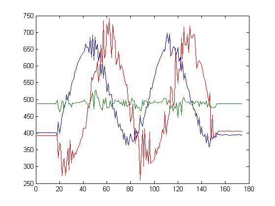
Rotated 720 Degrees Counter-Clockwise:

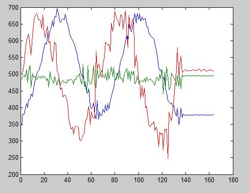
The green line shows little movement because the rotation of the acceleromter is calculated on a 3D scale and that is the axis in which it did not move in.

Team "FTQ": What can you find out from Bio80 notes or from the Internet about the normal range of exhaled CO2 percent in adult humans? Is that the percentage an anesthesiologist keeps a paralyzed patient at? What is the percentage of oxygen in the atmosphere at 4000m = 12000 ft elevation, compared to sea level?