Automatic Control
If the sampling theorem would be the single most important fact
you remember from EN123, then automatic control would be the most important
theme. Automatic control subsumes the ideas of feedback and feed-forward control;
negative and positive feedback, and particularly requires that the "plant"
being controlled exhibits some dynamics worth dealing with in the frequency
domain, likely by Laplace transform. On the other hand, the linear world of
Laplace transforms may be left behind confronting non-linear systems.
Examples of feed-forward control: audio
AGC (automatic gain control), mufflerless exhaust, fetal heart monitor...
0The varieties of feedback experience
As engineers we want to move beyond a hand-waving verbal account of feedback,
to a mathematical description which will allow us to model and predict various
actions of negative feedback controllers. This lecture introduces the context
of feedback and tells you about the virtues of feedback in any system. You'll
learn how feedback can stabilize, speed up and regulate a system. Part of what
you'll learn is terminology: feedback vs feedforward, negative vs positive feedback,
discrete vs continuous and linear vs nonlinear feedback.
Background: Recall
Laplace transforms from Circuits and Differential Equations courses.
Use Mathworks program SIMULINK to build
dynamic systems with feedback. A SIMULINK demo may be given for a nonlinear feedback
system. Simulink is like LabVIEW: An iconic language, with a wiring tool to make
connect icons.
%------------------------------------------
Feedback means sending a copy of an output signal
back to an input summation part of the system, where it can influence the system
components which helped form it in the first place. If this definition sounds
circular, it is! It may remind you of recursion in programming. The copy of
output sent as feedback may be attenuated or amplified; it may even be reversed
in sign. In any physical system the feedback path is inevitably associated with
some delay. The dynamics of that delay can create some of its most useful or
destabilizing effects. In the diagram below a summation unit adds external input
to output transformed through a feedback circuit. The effect of feedback may
be positive or negative at the summation point.
The summation point can be an op amp configured as a summation amplifier. The
forward pathway has two parts: The Plant is the apparatus itself--muscle, reactor
vessel, oven, motor, etc.--generally the Plant is not amenable to adjustment.
Compensation is where your design skills come in. Compensation will have gain
and possibly phase-shifting (filtering). In the feedback path is the SENSOR:
and it may translate a physical parameter such as temperature or air flow into
a voltage, so the SET point sees commensurable inputs.
Negative feedback is useful in various situations
where an output should be maintained at a desired level in spite of parameter
or load disturbances.
Automatic Control vs Homeostatics:
Automatic control is imagined to be
carried out by sensors that transduce physical data into voltage; control itself
is achieved by motors, heaters, pumps, and other electromechanical devices.
To account for sensing and control by biological tissue and organs, physiologists
(see Bio 80) use the term homeostatics. It implies that important physiological
parameters need to be kept in limited ranges, by means of negative feedback.
Examples are
Blood presssure (vessel dilation)
Blood sugar (insulin)
Potassium ions (actions in kidney)
Pupil diameter of the eye (light level)
Sense of balance (vestibular organ)
Temperature (metabolism)
Stretch reflex (golgi tendon organs)
Intracellular cyclic GMP (phosphodiesterase enzyme activity)
Closed loop gain calculation
Shown below are feed-forward and feedback configurations, with subtractive comparisons
at the summation units.
Now we develop the basic feedback equation, using algebra. The
compensation and plant have been combined into one forward path unit, G. Assume
a system output y(t) is intended to match a goal x(t), shown in
the figure below.
Without feedback y(t) = g(x(t)), where g is called gain and is a function-anything
from multiplication by a constant to a differential equation. With negative feedback
an error = x-f' is amplified by gain g until the negative feedback
reduces error to an acceptable level. The feedback signal is formed as the product
of y�f, where f is the feedback gain and f' is the feedback
signal presented to the summation amplifier on the left.
It's negative feedback because of the subtraction of f from goal
x.
Note that closed loop gain is lower than open loop gain. In fact
if f=1, closed loop gain is always less than 1! This reduction in gain had better
be good for something!
Virtues of negative feedback
1. Reduce sensitivity to internal parameter
changes
Suppose g = 100 in the system above. Then the close loop gain
is
Now suppose g changes by a factor of 2, to 200. The close loop gain is still
about 0.99. Negative feedback reduces sensitivity of the system to changes in
internal parameters. In this case the only internal parameter we have is open-loop
gain. What could make the system sensitive to gain changes? If the gain is too
low, less than 10 for example. In general, a high open loop gain is desired.
2. Reduce sensitivity to external
load changes
Let a variable load affect the output, as shown below:
Now
If L = 0 then the same G/(1+G) closed loop gain results. Even if L is not = 0, the
effect of load on the output is reduced by 1/(1+G) ! Thus negative feedback systems
have reduced sensitivity to external load changes. As an example of external load,
consider a beaker held up by the neuromuscular system of the arm; the aim is to
hold the beaker at a constant position in spite of liquid being poured in.
Example of plant and load dynamics: Suppose the
plant is a LP filter (leaky integrator)
Now suppose the load changes suddenly, at t=0, from 0 to 2: that would be
a step of magnitude 2:
and for t > 0 the output is close to 2/10, which would be the
(Load 2) / (Gain 10)
3. Increased speed of response
Now consider dynamics in the Plant. See the negative feedback system shown below.
Forward path and feedback are represented by Laplace transforms, so multiplication
of transfer functions can take the place of time-domain convolution integrals. Let

a "gain-of-one" first-order LP system.
[Review: What function of time
is this a transform of? What differential equation does the Laplace transform represent?
A leaky integrator, or first order LP filter.]
Let feedback be f = k, where k is attenuation: 0 < k < 1.
If F(s) = 1 then the open loop response of the system is Y(s) = In(s) � G(s).
If In(s)=1 (impulse function) then
a decaying exponential with time constant 1/a. The larger a is, the faster the system
decays. And decay to zero is what we want, when the input is an impulse. The impulse
is a brief disturbance, and we want the system to return to its zero state as soon
as possible. After t=0 input is zero, and we want y(t) to track the input. Now consider
the closed loop.
Substitute G(s) in the formula G/(1+G), which we can do because we
are in the frequency domain. If we were in the time domain, convolution would be
called for. At any rate, the formula simplifies to
which has inverse Laplace transform
Compared to the open loop form the time constant 1/(a+1) is smaller, so the system
decays to zero faster.
Suppose F>1 or GOL > 1 then
the time constant will be even smaller. Bottom line: Negative feedback can speed
up the response of a dynamic system.
(2009) Negative feedback, second order
systems, increased speed of response and underdamped responses. Imagine
the "plant" is something like an eyeball, and has rotational inertia,
viscous drag, and torsional spring stiffness of the antagonist muscle, modelled
in Laplace transform...
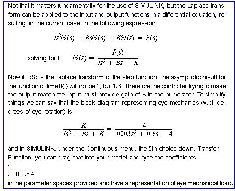
which is a v. overdamped dynamic system.
Consider a barely-overdamped transfer function, started by the following sequence,
shown "live" in lecture in Simulink...
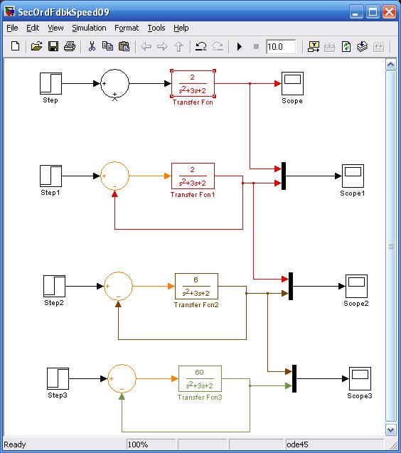
You will see that as the speed of response
increases the system becomes more underdamped, producing an undesirable oscillation
around the asymptotic value. Eventually compensation can artifically increase
damping and create speed increase without oscillation.
4. Stabilize a system
Now consider an unstable dynamic system:

Give the open loop block a Laplace transform with a negative time constant and set
feedback F = 0. The inverse Laplace transform is
The exponential is positive. The system is unstable. It's impulse response grows
exponentially. Now consider what happens if negative feedback is put in place. Let
F=1. Substituting in the basic formula we obtain
Let IN(s) be 1, for the input to be an impulse function. Now output is
A stable form with a decaying exponential. What's the time constant?
Bottom line here: Negative feedback can stabilize a system. Add
to the list of negative feedback virtues. Notice that in the dynamic examples given,
we haven't used large open loop gain, but certainly large open loop gain can amplify
the speeding-up and stabilizing effects
5. Inverse systems in feedback
Place the dynamic element in the feedback path, while maintaining a high open loop
gain A :
Applying the feedback formula
to this arrangement, while
letting IN(s) be 1, for the impulse input, we find,
If A*F(s) >> 1 then
So the element F(s) is turned
into its inverse: In a gyrator circuit a capacitor in a feedback loop "turns
into an inductor", for the sake of filter sharpness. In other cases we seek
the inverse of a system in order to "cancel" some effect or other.
Increasing first order LP time constant with positive feedback
Look at a dynamic system with positive feedback k less than 1:
Apply the feedback formula to find
OK, let's say k
< a. If
so, then a-k is a positive number smaller than a.
So the time constant of the system, 1/(a-k), is correspondingly larger
than 1/a.
Positive feedback can be used to "slow down" a leaky integrator.
Example: "Velocity
storage" in the VOR: lengthening the time constant of the vestibular apparatus,
from 5 sec to 20 sec. see
http://www.engin.brown.edu/courses/122JDD/Lcturs/vstopt05.html
where a positive feedback loop is embedded in an overall negative feedback loop
for visual tracking and fixation.
Push-Pull amplifier: Another example of two negatives
in a control loop creating positive feedback-- A push pull amplifier can accept
two inputs, sometimes out of phase with each other, such as vestibular nuclei
that are cross-coupled. Below is a diagram of a push pull system, with two internal
outputs subtracted for one external output. The gain equation is worked out:
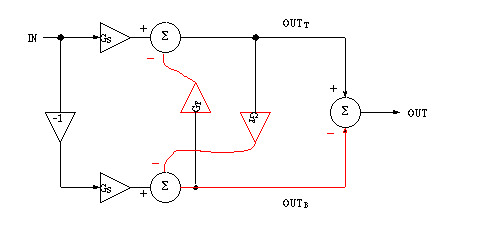
Notice that if GF is 0.9 then the gain is 20*Gs.
Transport delay in feedback path, plus an inverter for the plant
= oscillator. For now consider the the effect of delay in the one-inverter-with-feedback:
OUT becomes IN almost instantly, in "rise time" σ but IN must wait
a longer transport time Δ before it starts to change to the new value of IN.
Assume &Delta > σ. The result is the following "timing diagram"
for input and output waveforms. Thinking about what causes what can send you around
in circles, so start by considering that the circuit has just been turned on, and
IN is zero. As soon as power is applied, OUT goes (with rise-time sigma) to HI,
but a change of IN to HI must wait for delay Delta to expire.
An oscillation, with period 2�(Delt+sig), results.
[If sig > Delt, then the metastable condition can last "a long time";
such may be the case with various IC inverters.]
(To be more careful in this analysis of feedback we must specify the thresholds
2H
and 2L
at which the inverter snaps from one binary value to another.
Assume for now that
OUT will snap up if IN < 1 volt = θL, and
OUT will snap down if IN > 4 volts = θH .
Delay in feedback The Laplace transform of pure delay is:
An example: The signal going up from a spindle to a motoneuron
in a feedback loop is not just slowed down by an integration process, it is absolutely
delayed by finite (and slow) conduction speed. In engineering terms such delay is
called transport delay. It's commonly seen is chemical engineering
systems where fluid to be measured (dissolved electrolyte, for example) is transported
down a pipe until it arrives at a sensor. How can we handle pure delay in terms
of Laplace transforms? The Laplace transform of pure delay f(t-t0) is exp(-s*t0)*F(s)
where t0 is the duration of the transport delay. The exponential can be approximated
by the Maclaurin series,
Without having to work out an analytical solution, we can demonstrate the effect
of transport delay with SIMULINK (an efficient way to simulate dynamic systems)
from Mathworks, up the road in Natick, MA.
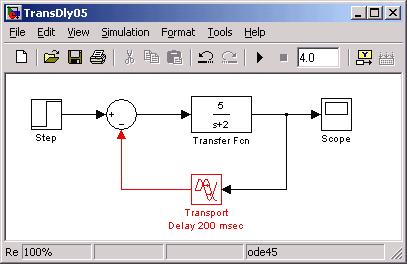
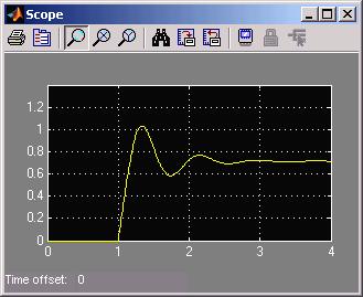
where you see that a first order system now appears like a second order underdamped
response due to transport delay in the feedback path.
Proportional, integral, derivative compensation
Control engineers call it PID. So far we have considered mainly proportional
compensation, where the error signal is multiplied by some proportional factor,
KP. We will look briefly at the effects of PID compensation. For example, integral
feedback is capable of driving the error of a system to zero, not just to some small
value. Follow the development in Wolovich's book, pages 271-286.
PI controller: Proportional + Integral compensation looks like
which has the form (in EN122, eye movements) of the Oculomotor Nucleus compensation
before the transfer function representing eyeball mechanics.
Example of Integral compensation driving error to zero. Start
with the Simulink model shown below, with a first order plant having a low frequency
open loop gain of 5:
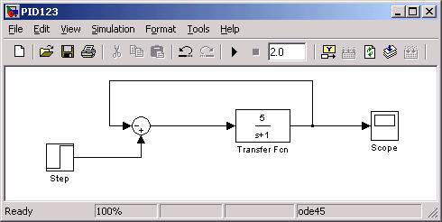
Below is the Scope output for a step input start at t = 0.5.
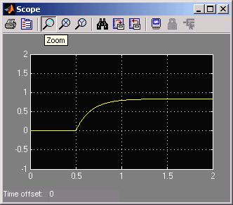
Notice the permanent error of 1/6 from the desired output of 1.00. G/(1+G) = 5/6.
Now add integral compensation:
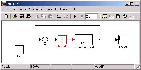
We can start to work out what we expect analytically at the output: The close loop
transfer function is
The integral compensation has taken the system to 2nd order, and an underdamped
2nd order at that. Remembering that the Laplace transform of the step input is 1/s,
we see that output is
a partial fraction expansion that can be solved for the coefficients A0, A1, A2.
We will expect as a function of time a step and damped oscillation. See the Simulink
output below:
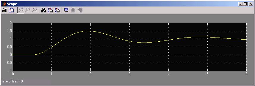
Which has the expected damped oscillation of period 2.88 seconds. Notice that the
asymptotic value is now 1.00. No error! Yes, there are oscillations leading up to
the approach to the exact answer: that would be expected of something converted
to an underdamped second order system.
Feb 2005: Numerical solution for PFE coefficients of the step
component of response: Use Matlab function residue to find coefficients
of PFE for proportional and integral compensation of example above:
>> help residue
>> Ai = [ 1 1 5 0 ] % coefficients
of integral control response
>> B = 5
>> [R,P,K] = residue(B,Ai)
with the result that the "residue"
or PFE coefficient of C/s is C = 1.0.
Since the inverse Laplace transform of C/s is C*1(t), where 1(t) is the step
response, then the steady-state response to integral control is perfect match
to a 1/s step input.
When we consider proportional
control then the closed-loop proportional output response to a step input is:
And the proportional coefficients
AP = [ 1 6 0 ]
calculating residues in Matlab:
>> [R,P,K] = residue(B,Ap)
with the result that now the "residue"
of C/s is C = 0.8333 = 5/6 and 1-5/6 = .16666 is the steady-state error of proportional
control.
Proportional-Derivative
compensation  is
more problematical: To quote from Wolovich (p.281): "In general, an ideal
derivative compensator is difficult to construct (exception: a tachometer).
Moreover, since its magnitude increases without bound as frequency increases,
an ideal differentiator produces undesirable amplification of any high frequency
noise that may be present in the loop." Practical derivative control needs
a leaky integrator to eliminate high frequency instability.
is
more problematical: To quote from Wolovich (p.281): "In general, an ideal
derivative compensator is difficult to construct (exception: a tachometer).
Moreover, since its magnitude increases without bound as frequency increases,
an ideal differentiator produces undesirable amplification of any high frequency
noise that may be present in the loop." Practical derivative control needs
a leaky integrator to eliminate high frequency instability.
---------------------------- --------------------------------
Bang Bang controller: Up to now we have considered the
error signal as a "floating point" number whose magnitude and sign are
used to tell the plant how to best to correct the error; the first-order attempt
by the plant is a proportional response. What if there is a region of error we don't
care about, and beyond the don't-care region we want the controller to work at a
constant (perhaps maximum) rate? Then we want a bang-bang controller.
When a bang-bang system senses a signal is out of range it
turns on the controller to a "maximum" setting until the signal comes
back in range, then it turns the controller off completely. The controller may
have 2 maximum settings, such as hot/cold, or CW/CCW. By "out of range"
we mean that there is a hysteresis range within which the output tolerated:
The narrower the range, the more frequently the controller will turn on and
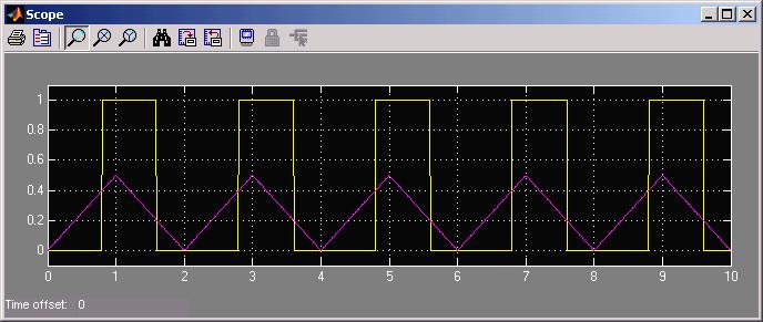
off (turning the furnace on and off for example). Below we show a Simulink model
for a bang-bang controller, and its output due to a triangle-wave input:
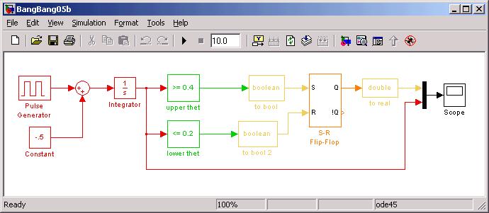
The red part on the left above generates the triangle wave shown below in purple.
In the diagram above it is necessary to convert from Boolean to floating point
(yellow boxes). The memory element in the controller is the Set-Reset Latch,
shown in orange.
The hysteresis thresholds for turning the controller on and off are 0.2 and
0.4. If the input is rising, it turns on the controller above 0.4, but doesn't
turn it off again until the input is less than 0.2.
The excitation table for a S-R latch is
| Set |
Reset |
Q |
| 0 |
0 |
no change |
| 0 |
1 |
0 |
| 1 |
0 |
1 |
| 1 |
1 |
NOT ALLOWED |
where the state SR = 00 is the memory state, whose output depends on previous input
timing.
See Daniels, Digital Design From Zero to One, chpt 5, John Wiley & Sons
(1996) for more details about flip flops and latches.
The Simulink example above is lacking two important features:
1. There is no feedback in the model!
2. There is no dynamics!
The model illustrates hysteresis by bang-bang control, that's all. .
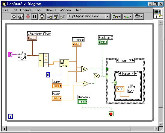
LabVIEW (EN123) can also support bang-bang controllers, but LabVIEW
does not have SR latches as such; it relies on logic for exiting from While
loops, as this example shows.
In the next example ( linked at bang-bang
heater) we provide dynamics from the thermal properties of a body being
heated, and close the feedback loop, with cool ambient temperature as a parametric
input to the plant.
Fuzzy Logic Controller. The interval of acceptable
output can be better described by a bell-shaped or triangle-shaped function,
and called a fuzzy set membership function. (more later... See Bart Kosko, Fuzzy
Engineering, P-H (1997): Part III, "Fuzzy Control and Chaos".)
To see fuzzy logic in action, with Simulink, go to the Fuzzy
Logic Toolbox documentation and find the water level control example: here
is the path--
Help:Fuzzy Logic Toolbox:Tutorial:Working with Simulink:An Example-Water Level
Control
Demo: Balancing a 1m PVC pipe on my palm: moving feet
not allowed; visual feedback: monocular: nondominant eye only; looking at hand
instead of pole; in strobe light, 10Hz.
Regulation of air flow (EN123 Lab)
Show OUT = BIAS + Reg(s) as output air flow.
(What is the nonlinear relationship between voltage and flow velocity?)
Reg(s) is the output of E(s*M(s) where E is the error, E = Set - F(s)OUT and M(s)
is the fan characteristic Set is the desired airflow OUT(s) goes to T(s) the tach
and perhaps gain or C(s), compensation. Gain may be needed in the "open loop"
We end up with an equation
(demonstrates regulation of Bias type noise...)
If you're using LabVIEW you want OUT to equal SET; IN-OUT is the error.
Adaptive gain control. (2006) There are really two ways to react to error
signals: One: What we have seen so far: let the increased error itself be the
input to the plant (negative feedback); or Two: Have the "unconditioned stimulus"
be the input and let the error control a process that changes the gain itself.
This second approach is called adaptive gain control and is the basis of adaptive
neural networks, a topic itself large enough for a one-semester course. Below
is a Simulink model of a 1-input adaptive gain controller, and the relevant outputs:
(EN122: needed for adaptive gain control of VOR)
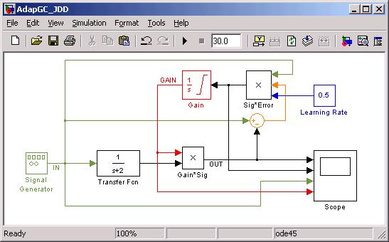
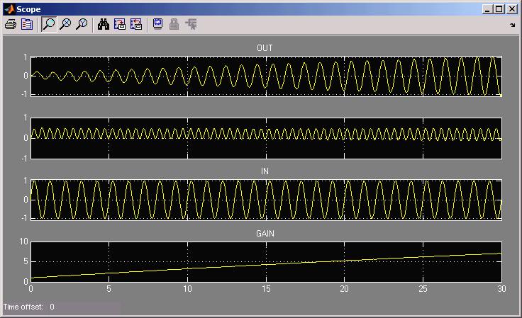
See link to Notes on Gradient
Descent to see why three signals:
Learning Rate*Error*Stimulus, are multiplied together for Gain integrator input. Notice
that the change in gain is "permanent": if the input goes to zero, the integrator
retains its new value...long-term memory. More detail below:
The equations unfortunately do not boil down to something as straightforward as
OUT = G/(1+G)*IN, but are amenable to simulation, where weight W(t) is the output
of an integrator whose input is the product of the three factors shown.
Suggested Reading
W. A. Wolovich Automatic
Control Systems, Saunders (1993), "PID Compensation,"
pages 271-286.
Curtis D. Johnson, Process
Control Instrumentation Technology
7th Edition, Prentice-Hall (1998).
Other Reading
Clare D. McGillem & G.R. Cooper, chapter 5, �15, "Feedback systems,"
pages 270-283, in Continuous and Discrete Signal and System Analysis,
3rd Edition, Holt-Rinehart and Winston (1991).
V. S. Vaidhyanathan, Regulation
and Control Mechanisms in Biological Systems, Prentice-Hall (1993).
Oppenheim & Willsky, chapter 11 (first 2 �'s) pages 685-701
in Signals and Systems, Prentice-Hall (1983). O&W was the
EN157 book a few years ago.
Summary
* G-CL = G/(1+G) where G is open-loop gain
* G/(1+FG), where F is feedback gain.
If FG>>1 then an inverse system F-inv can be created at output
* Virtues of negative feedback
insensitivity to parameter or load changes
increased speed
improves stability
* Creating inverse systems
* Positive feedback gain-less-than-one to increase time constant
* Frequency response as a function of loop gain.
* Delay & stability & non-linear/time varying systems
* PID = proportional/derivative/differential compensation
& the problem of pure differentiation
* Bang-bang controllers
* Fuzzy logic controllers
* Adaptive gain control (neural networks)