Chapter 12

 

Dynamic solutions for elastic solids

 

 

 

In this section we discuss briefly the motion of elastic solids subjected to some loading.   We will consider two topics: (1) wave propagation in an elastic solid; and (2) vibrations.

 

 

12.1 Wave propagation in a string

 

We can develop some physical intuition into how deformable solids will move by solving some simple problems.   We start by analyzing motion of strings $–$ these are simple $–$ but it turns out that waves in a string behave the same way as plane waves in an elastic solid.

 

Example 1: Traveling wave propagation in a stretched string with given initial conditions

 

We can learn a lot about the behavior of waves in solids by looking at the behavior of a stretched string. For this purpose we solve the following problem:  An infinitely long string under axial tension $T_0$ as at rest and has a transverse displacement

$u_1(x_3)=u^{(0)}(x_3)$

at time t=0.   Find the subsequent motion of the string.

 

We derived the governing equation for a string in Chapter 10.  It is

$T_0\frac{d^2{u}_1}{d{x}_3^2}=\rho A\frac{d^2{u}_1}{d{t}^2}\Rightarrow \frac{d^2{u}_1}{d{x}_3^2}=\frac{1}{c^2}\frac{d^2{u}_1}{d{t}^2}$

 where  $c=\sqrt{T_0/\rho A}$ is the wave speed.

 

This is the famous wave equation.   It has a rather simple general solution $u_1=f(x_3-ct)+g(x_3+ct)$ where f and g are arbitrary functions, which must be determined from the initial conditions (and if the string has ends, boundary conditions at the ends).   For the current case the initial conditions for $u_1$ give

$f(x_3)+g(x_3)=u^{(0)}(x_3)\frac{\partial u_1}{\partial t}=-cf\text{'}(x_3)+cg\text{'}(x_3)=0$

where $f\text{'}(\lambda )=df/d\lambda ,g\text{'}(\lambda )=dg/d\lambda$ .   To solve these for f and g just integrate the second one, which gives us two equations

$f(x_3)+g(x_3)=u^{(0)}(x_3)-f(x_3)+g(x_3)=A$

where A is a constant.   Solve these

$f(x_3)=[u^{(0)}(x_3)-A]/2g(x_3)=[u^{(0)}(x_3)+A]/2$

So the solution is

$u_1(x_3)=f(x_3-ct)+g(x_3+ct)=[u^{(0)}(x_3-ct)+u^{(0)}(x_3+ct)]/2$

The solution (with initial condition $u(0,x_3)=\exp (-x_3^2/4)$ )  is animated in the figure below   

 

 

You can see the initial disturbance split into two waves, which propagate at stead speed down the string.  These are the functions f and g:  f  is a wave propagating to the right, and g is a wave propagating to the left.  Of course, the wave motion is just an illusion $–$ every point in the string moves transverse to its axis, but like the ‘wave’ in an athletic stadium the disturbance appears to propagate even though the crowd are just raising and lowering their arms.  

 

 

Example 2: Traveling wave propagation in a stretched string with prescribed motion at an end

 

The same general solution can be used to solve any traveling wave problem.  For example, suppose we hold one end of a very long string.  The string is at rest with $u_1=d{u}_1/dt=0$ everywhere at t=0.  We then move the end we are holding with a prescribed displacement $u^{*}(t)$ .   Find the displacement.

 

As before, the solution is $u_3=f(x_3-ct)+g(x_3+ct)$.  Note that $f(\lambda )$  must be calculated for all $-\infty <\lambda <\infty$, since for any $x_3$ its argument will be negative for sufficiently large t, but $g(\lambda )$ need only be defined for $\lambda >0$ , since its argument is never negative .The initial conditions give

$f(x_3)+g(x_3)=0cf\text{'}(x_3)-cg\text{'}(x_3)=0x{}_3\ge 0$

Integrate the second equation and then solve for f and,g to see that

$f(x_3)=A,g(x_3)=-A{x}_3\ge 0$

This gives us g everywhere we need it, and tells us $f(\lambda )$ for $\lambda >0$ .  We can find $f(\lambda )$ for $\lambda <0$ from the boundary condition on displacement at $x_3=0$

$f(-ct)+g(ct)=u^{*}(t)t\ge 0$

We already know $g(ct)=-At\ge 0$  so it follows that

$f(-ct)=A+u^{*}(t)t\ge 0\Rightarrow f(\lambda )=A+u^{*}(-\lambda /c)\lambda \le 0$ .

We now have the complete solution, which can be re-written as

$u_3(t,x_3)=\{\begin{array}{c}0x_3-ct>0\\ u^{*}(t-x_3/c)x_3-ct<0\end{array}$

It is a bit easier to visualize this if we re-write the conditional as

$u_3(t,x_3)=\{\begin{array}{c}0t-x_3/c<0\\ u^{*}(t-x_3/c)t-x_3/c>0\end{array}$

This equation says that every point on the string experiences the same history of displacement $u*$ , but a point at position $x_3$ will experience the displacement at a time $x_3/c$ later than the point at $x_3=0$ .  Of course we already know that, but it is nice to see the math work out.

 

The figure below animates the behavior of a string that has its leftmost end moved through two cycles  of a sin wave.

 

 

Example 3: Reflections at a boundary

 

Finally, we look at what happens when a wave reaches the end of a string.  The figure shows the two possible types of boundary: at $x_3=L$ is a fixed end; $x_3=-L$ is a free end.   The string is at rest at time t=0 and has a transverse displacement

$u_1(x_3)=u^{(0)}(x_3)$

For simplicity we assume that the string is only displaced near the origin, and in particular $u^{(0)}(x_3)=0$ at $x_3=\pm L$ .

 

The two boundary conditions at the ends are

$u_1=0x_3=L\frac{d{u}_1}{d{x}_3}=0x_3=-L$

We can satisfy these by extending the string to $\pm \infty$ , and introducing initial displacements into the imaginary parts of the string outside $-L<x_3<L$ that will satisfy the two boundary conditions.  Hopefully you can see that to cancel the forward propagating wave (to keep the end fixed at $x_3=L$ ) you need to introduce an initial displacement in the opposite direction centered at $x_3=2L$ , while to keep the slope fixed at $x_3=-L$ , you need to introduce a disturbance of the same sign at $x_3=-2L$ .   The figure below illustrates the idea graphically: the waves generated by the initial displacements of the fictitious blue parts of the string will reach the boundaries at just the same time as those in the real, brown parts: on the right, the waves cancel and give zero displacement; on the left, they combine and keep the slope zero.

Of course the process does not end here: we need to continue extending the string to both left and right and add the appropriate initial displacements to satisfy boundary conditions at the two ends for all time.  The animation below shows the full sequence (the left end is free; the right end is fixed).  If you enjoy puzzles and some basic matlab coding you might find it instructive to try to reproduce the result yourself.

You can watch the two ends to understand the two types of reflection:

·         At a fixed end, a wave with positive deflection reflects as one with a negative deflection;

·         At a free end, a wave with positive deflection reflects as one with a positive deflection sign.

 

It is helpful to understand how reflections influence transverse forces in the string as well.   Recall that the transverse force in a string is related to the deflection by

$T_1=T_0\frac{d{u}_1}{d{x}_3}$

An animation of the transverse force is shown below

 Watch the animation and convince yourself that

·         At a fixed end, a positive transverse force is reflected as a positive transverse force;

·         At a free end, a positive transverse force is reflected as a negative transverse force.

The rules governing reflections of forces are the opposite to those governing displacement.

 

 

 

12.2: Pressure and shear plane waves in 3D elastic solids

 

Now that we understand strings, we can think about waves in 3D elastic solids.   Start with the special case of an infinitely large, isotropic linear elastic solid with Young’s modulus E, Poissons ratio $\nu$ and mass density $\rho$ that fills all of space.   Consider motion of the form

$u(x,t)=u_1(x_3,t)e_1+u_3(x_3,t)e_3$

This describes a so-called ‘plane wave’ that propagates in the $x_3$  direction.  To visualize the motion note that

(1)   every point that lies in a particular $(x_1,x_2)$ plane has the same displacement

(2)   $u_1(x_3)$ is a displacement transverse to the propagation direction (a so called ‘Shear wave’ or S-wave).  This is just like the motion of a wave moving along a string.

(3)   $u_3(x_3)$$–$ it is a displacement parallel to the wave propagation direction (a ‘Pressure wave’ or P-wave).   This type of motion can’t occur in a string, but it does occur in long flexible springs (like a slinky) which can be stretched axially.

 

We can now substitute this displacement field into the elasticity equations:

 The strain-displacement relation gives

${\epsilon }_{13}=\frac{1}{2}\frac{\partial u_1}{\partial x_3}{\epsilon }_{33}=\frac{\partial u_3}{\partial x_3}$

 The elastic stress-strain law gives

$\begin{array}{l}{\sigma }_{33}=\frac{E(1-\nu )}{(1+\nu )(1-2\nu )}{\epsilon }_{33}=\frac{E(1-\nu )}{(1+\nu )(1-2\nu )}\frac{\partial u_3}{\partial x_3}\\ {\sigma }_{13}=\frac{E}{(1+\nu )}{\epsilon }_{13}=\frac{E}{2(1+\nu )}\frac{\partial u_1}{\partial x_3}\end{array}$

 Finally, the linear momentum balance equation gives

$\begin{array}{l}\frac{\partial {\sigma }_{33}}{\partial x_3}=\rho \frac{{\partial }^2{u}_3}{\partial t^2}\Rightarrow \frac{{\partial }^2{u}_3}{\partial x_3^2}=\frac{1}{c_L^2}\frac{{\partial }^2{u}_3}{\partial t^2}\\ \frac{\partial {\sigma }_{33}}{\partial x_3}=\rho \frac{{\partial }^2{u}_1}{\partial t^2}\Rightarrow \frac{{\partial }^2{u}_3}{\partial x_3^2}=\frac{1}{c_s^2}\frac{{\partial }^2{u}_3}{\partial t^2}\end{array}$

 

where

  $c_L^{}=\sqrt{E(1-\nu )/\rho (1+\nu )\left(1-2\nu \right)}$ is the speed of longitudinal wave propagation through the solid

  $c_s=\sqrt{E/2(1+\nu )\rho }$ is the speed of shear wave propagation through the solid.

 

The longitudinal wave is always faster than the shear wave.

 

These are the same wave equation that governs the motion of a string.  Everything we learned about strings applies without modification to plane waves in 3D elastic solids.

 

Example 1: An isotropic, linear elastic half space with Young’s modulus E, Poisson’s ratio $\nu$ and mass density $\rho$ occupies the region $x_3>0$ .  The solid is at rest and stress free at time t=0.  For t>0 it is subjected to a pressure p(t) on $x_3=0$ as shown in the picture. 

Solution: The displacement and stress fields in the solid (as a function of time and position) are

$\begin{array}{l}{u}_3(x_3,t)=\{\begin{array}{c}\frac{c_L}{E}\frac{(1+\nu )(1-2\nu )}{(1-\nu )}{\displaystyle \underset{0}{\overset{t-x_3/c_L}{\int }}p(\tau )d\tau x_3<t{c}_L}\\ 0x_3>t{c}_L\end{array}\\ {\sigma }_{33}=\{\begin{array}{c}-p(t-x_3/c_L)x_3<t{c}_L\\ 0x_3>t{c}_L\end{array}\end{array}$

where $c_L^{}=\sqrt{E(1-\nu )/\rho (1+\nu )\left(1-2\nu \right)}$ is the speed of longitudinal wave propagation through the solid.  All other displacement and stress components are zero.  For the particular case of a constant (i.e. time independent) pressure, magnitude ${\sigma }_0$, applied to the surface

$u_3(x_3,t)=\{\begin{array}{c}\frac{(1-2\nu )(1+\nu )}{(1-\nu )}\frac{{\sigma }_0}{E}(c_{L}t-x_3)x_3<c_{L}t\\ 0x_3>c_{L}t\end{array}$              ${\sigma }_{33}=\{\begin{array}{c}-{\sigma }_0{x}_3<c_{L}t\\ 0x_3>c_{L}t\end{array}$

Evidently, a stress pulse equal in magnitude to the surface pressure propagates vertically through the half-space with speed $c_L$.

 

Notice that the velocity of the solid is constant in the region $0<x_3<t{c}_L$, and the velocity is related to the pressure by

$v_3=c_L\frac{(1-2\nu )(1+\nu )}{(1-\nu )}\frac{{\sigma }_0}{E}=\frac{{\rho }_0}{c_L}{\sigma }_0$

 

Derivation: The solution can be derived as follows.

 

1.      The solution to the 1-D wave equation is

$u_3(x_3,t)=f(t-x_3/c_L)+g(t+x_3/c_L)$

where f and g are two functions that must be chosen to satisfy boundary and initial conditions.

2.      The initial conditions are

$\begin{array}{c}{u}_3(x_3,0)=f(-x_3/c_L)+g(x_3/c_L)=0\\ \frac{\partial u_3}{\partial t}=f^{\prime }(-x_3/c_L)+g^{\prime }(x_3/c_L)=0\end{array}\}{x}_3\ge 0$

where the prime denotes differentiation with respect to its argument.  Solving these equations shows that

$f(-x_3/c_L)=-g(x_3/c_L)=A$

where A is some constant.

3.      Observe that $t+x_3/c_L\ge 0$ for t>0, so that $g(t+x_3/c_L)=-A$.  Substituting this result back into the solution in (4) gives $u_3(x_3,t)=f(t-x_3/c_L)-A$.

4.        Next, use the boundary condition ${\sigma }_{22}=-p(t)$ at $x_3=0$ to see that

$\begin{array}{l}{\sigma }_{33}=\frac{E(1-\nu )}{(1+\nu )(1-2\nu )}\frac{\partial u_3}{\partial x_3}=-p(t)\Rightarrow \frac{E(1-\nu )}{(1+\nu )(1-2\nu )}\left(\frac{-1}{c_L}\right)f\text{'}(t)=-p(t)\\ \Rightarrow f(t-x_3/c_L)=\frac{c_L}{E}\frac{(1+\nu )(1-2\nu )}{(1-\nu )}{\displaystyle \underset{0}{\overset{t-x_3/c_L}{\int }}p(\tau )d\tau }+B\end{array}$

where B is a constant of integration.

5.      Finally, B can be determined by setting t=0 in the result of (7) and recalling from step (5) that $f(-x_3/c_L)=A$.  This shows that B=-A and so

$\begin{array}{l}{u}_3(x_3,t)=\frac{c_L}{E}\frac{(1+\nu )(1-2\nu )}{(1-\nu )}{\displaystyle \underset{0}{\overset{t-x_3/c_L}{\int }}p(\tau )d\tau }\\ {\sigma }_{33}=-p(t-x_3/c_L)\end{array}$

as stated.

 

 

Example 2: Surface subjected to time varying shear traction

An isotropic, linear elastic half space with Youngs modulus E and Poisson’s ratio $\nu$ and mass density $\rho$ occupies the region $x_3>0$ .  The solid is at rest and stress free at time t=0.  For t>0 it is subjected to a uniform anti-plane shear traction p(t) on $x_3=0$.  Calculate the displacement, stress and strain fields in the solid.

 

It is straightforward to show that in this case

$u_1(x_2,t)=\frac{2(1+\nu )c_s}{E}{\displaystyle \underset{0}{\overset{t-x_3/c_s}{\int }}p(\tau )d\tau }$

${\sigma }_{31}=-p(t-x_3/c_s)$

where $c_s^2=\frac{E}{2(1+\nu )\rho }$ is the speed of shear waves propagating through the solid.  The details are left as an exercise.

 

 

Example 3: 1-D Bar subjected to end loading

 

This solution is a cheat, because it doesn’t satisfy the full 3D equations of elasticity, but it turns out to be quite accurate.

 

A long thin rod occupying the region $x_1>0$ is made from a homogeneous, isotropic, linear elastic material with Young’s modulus E and mass density ${\rho }_0$.  At time t<0 it is at rest and free of stress.  At time t=0 it is subjected to a pressure p(t) at one end.  Calculate the displacement and stress fields in the solid.

 

We cheat by modeling this as a 1-D problem.  We assume that ${\sigma }_{11}$ is the only nonzero stress component, in which case the constitutive law and balance of linear momentum require that

$\begin{array}{l}{\sigma }_{11}=E\frac{\partial u_1}{\partial x_1}\frac{\partial {\sigma }_{11}}{\partial x_1}={\rho }_0\frac{{\partial }^2{u}_1}{\partial t^2}\\ \Rightarrow \frac{{\partial }^2{u}_1}{\partial x_1{}^2}=\frac{1}{c_B^2}\frac{{\partial }^2{u}_1}{\partial t^2}\end{array}$

where $c_B^2=E/{\rho }_0$ is the wave speed. This equation is exact for $\nu =0$ but cannot be correct in general, since transverse motion is neglected.  In practice waves are repeatedly reflected off the sides of the bar, which behaves as a wave-guide.

 

 It is straightforward to solve the equation to see that

$u_1(x_2,t)=\frac{c_B}{E}{\displaystyle \underset{0}{\overset{t-x_1/c_B}{\int }}p(\tau )d\tau }$

${\sigma }_{11}=-p(t-x_1/c_B)$

 

 

 

Summary of Wave Speeds in isotropic elastic solids.

 

It is worth summarizing the three wave speeds calculated in the preceding sections.  Recall that

                            $c_L^2=\frac{E(1-\nu )}{{\rho }_0(1+\nu )(1-2\nu )}=\frac{2\mu (1-\nu )}{{\rho }_0(1-2\nu )}{c}_s^2=\frac{E}{2(1+\nu ){\rho }_0}=\frac{\mu }{{\rho }_0}{c}_B^2=\frac{E}{{\rho }_0}$

It is possible to show that, for all positive definite materials (those with positive definite strain energy density $–$ a thermodynamic constraint) $c_L>c_S$.  For most real materials $c_L>c_B>c_s$.

 

There are also special kinds of waves (called Rayleigh and Stoneley waves) that travel near the surface of a solid, or near the interface between two dissimilar solids, respectively.  These waves have their own speeds.  Rayleigh waves are discussed in more detail in Section 11.3 below.

 

 

Reflection of waves traveling normal to a free surface

 

Suppose that a longitudinal wave with stress state

$\begin{array}{l}{u}_1(x_1,t)=-\frac{c_L}{E}\frac{(1+\nu )(1-2\nu )}{(1-\nu )}{\displaystyle \underset{0}{\overset{t-x_2/c_L}{\int }}f(\tau )d\tau }\\ u_2=u_3=0\\ {\sigma }_{11}=f(t-x_1/c_L)\end{array}$

is incident on a free surface at $x_1=a$.  Calculate the state of stress in the solid as a function of time, accounting for the stress free surface.

 

To visualize the wave, imagine that it is a front, such as would be generated by applying a constant uniform pressure at $x_1=0$ at time t=0.  The material ahead of the front is at rest, and stress free, while behind the front material has a constant stress and velocity. 

 

At time $t=a/c_L$ the front would reach the free surface and be reflected.  Let the horizontal stress associated with the reflected wave be

${\sigma }_{11}=g(t+x_1/c_L)$

(we need a + in the argument because the wave travels to the left and has negative velocity). For the stress to vanish at the free surface, we must have

$f(t-a/c_L)+g(t+a/c_L)=0$

so,

$g(t+x_1/c_L)=-f(t-a/c_L+(x_1-a)/c_L)$

and the full solution consists of both incident and reflected waves

$\begin{array}{l}{u}_1(x_1,t)=-\frac{c_L}{E}\frac{(1+\nu )(1-2\nu )}{1-\nu }\left\{{\displaystyle \underset{0}{\overset{t-x_2/c_L}{\int }}f(\tau )d\tau }+{\displaystyle \underset{0}{\overset{t-a/c_L+(x_2-a)/c_L}{\int }}f(\tau )d\tau }\right\}\\ u_2=u_3=0\\ {\sigma }_{11}=f(t-x_1/c_L)-f(t-a/c_L+(x_1-a)/c_L)\end{array}$

 

 

        

 

As a specific example, consider a plane, constant-stress wave that is incident on a free surface. The histories of stress and velocity in the solid are illustrated in the figures above. In this case:

1.      Behind the incident stress wave, the stress is constant, with magnitude ${\sigma }_0$.   The velocity of the solid is constant, and related to the stress by $v_1=-\rho {\sigma }_0/c_L$

2.      At time $t=a/c_L$ the stress wave reaches the free surface.  At this time an equal and opposite stress pulse $-{\sigma }_0$ is reflected from the free surface, and propagates away from the surface.

3.      Behind the reflected wave, the solid is stress free, and, the solid has constant velocity  $v_1=-2\rho {\sigma }_0/c_L$

 

12.3 Rayleigh waves

A Rayleigh wave is a special type of wave which propagates near the surface of an elastic solid.  Assume that

 The solid is an isotropic, linear elastic material with Young’s modulus $E$, Poisson’s ratio $\nu$ and mass density ${\rho }_0$

 The solid has shear wave speed  $c_s$ and longitudinal wave speed $c_L$

 The surface is free of tractions

 A Rayleigh wave with wavelength $\lambda$ propagates in the $x_1$ direction

 

The nonzero components of displacement and stress in a Rayleigh wave are

$\begin{array}{l}{u}_1=\frac{U_{0}ik}{(k^2-{\beta }_T^2){\beta }_L}\exp \left(ik(x_1-c_{R}t)\right)\left\{(k^2+{\beta }_T^2)\exp \left(-{\beta }_L{x}_2\right)-2{\beta }_L{\beta }_T\exp \left(-{\beta }_T{x}_2\right)\right\}\\ u_2=\frac{U_0}{(k^2-{\beta }_T^2)}\exp \left(ik(x_1-c_{R}t)\right)\left\{2k^2\exp \left(-{\beta }_T{x}_2\right)-(k^2+{\beta }_T^2)\exp \left(-{\beta }_L{x}_2\right)\right\}\end{array}$

$\begin{array}{l}{\sigma }_{11}=\frac{U_{0}E\exp \left(ik(x_1-c_{R}t)\right)}{(k^2-{\beta }_T^2)(1+\nu )(1-2\nu ){\beta }_L}\{k^2\left[\nu ({\beta }_L^2+{\beta }_T^2)-(1-\nu )(k^2+{\beta }_T^2)\right]\exp \left(-{\beta }_L{x}_2\right)\\ +2k^2{\beta }_T{\beta }_L(1-2\nu )\exp \left(-{\beta }_T{x}_2\right)\}\\ {\sigma }_{22}=\frac{U_{0}E\exp \left(ik(x_1-c_{R}t)\right)}{(k^2-{\beta }_T^2)(1+\nu )(1-2\nu ){\beta }_L}\{(k^2+{\beta }_T^2)\left[(1-\nu ){\beta }_L^2-\nu k^2\right]\exp \left(-{\beta }_L{x}_2\right)\\ -2k^2{\beta }_T{\beta }_L(1-2\nu )\exp \left(-{\beta }_T{x}_2\right)\}\\ {\sigma }_{12}=\frac{i{U}_{0}kE(k^2+{\beta }_T^2)}{(k^2-{\beta }_T^2)(1+\nu )}\exp \left(ik(x_1-c_{R}t)\right)\left\{\exp \left(-{\beta }_T{x}_2\right)-\exp \left(-{\beta }_L{x}_2\right)\right\}\end{array}$

where $i=\sqrt{-1}$, $U_0$ is the amplitude of the vertical displacement at the free surface, $k=2\pi /\lambda$ is the wavenumber; ${\beta }_L=k\sqrt{1-c_R^2/c_L^2}$, ${\beta }_T=k\sqrt{1-c_R^2/c_s^2}$; and $c_R$ is the Rayleigh wave speed, which is the positive real root of

${\left(2-\frac{c_R^2}{c_s^2}\right)}^2-4{\left(1-\frac{(1-2\nu )}{2(1-\nu )}\frac{c_R^2}{c_s^2}\right)}^{1/2}{\left(1-\frac{c_R^2}{c_s^2}\right)}^{1/2}=0$

This equation can easily be solved for $c_R/c_s$ with a symbolic manipulation program, which will most likely return 6 roots.  The root of interest lies in the range $0.65<c_R/c_s<1$ for $-1<\nu <0.5$. The solution can be approximated by $c_R/c_s=0.875-0.2\nu -0.05{(\nu +0.25)}^3$ with an error of less than 0.6% over the full range of Poisson ratio.

 

You can use either the real or imaginary part of these expressions for the displacement and stress fields (they are identical, except for a phase difference). Of course, if you choose to take the real part of one of the functions, you must take the real part for all the others as well. Note that substituting $x_2=0$ in the expression for ${\sigma }_{22}$ and setting ${\sigma }_{22}=0$ yields the equation for the Rayleigh wave speed, so the boundary condition ${\sigma }_{22}=0$ is satisfied.  The variations with depth of stress amplitude and displacement amplitude are plotted below.

      

 

Important features of this solution are:

1. The wave is confined to a layer near the surface with thickness about twice the wavelength. 
2. The horizontal and vertical components of displacement are 90 degrees out of phase.  Material particles therefore describe elliptical orbits as the wave passes by.
3. The speed of the wave is independent of its wavelength $–$ that is to say, the wave is non-dispersive.
4. Rayleigh waves are exploited in a range of engineering applications, including surface acoustic wave devices; touch sensors; and miniature linear motors.  They are also observed in earthquakes, although these waves are observed to be dispersive, because of density variations of the earth’s surface.

 

Other similar kinds of wave occur in solids: waves near an interface between two dissimilar elastic solids are called ‘Stoneley’ waves.   There are also special kinds of waves that occur in thin layers, which behave like wave-guides.

 

12.4 Travelling waves in beams

 

 

We end our discussion of waves with a brief look at waves in beams, which show that many of the things we learn about waves in elementary courses aren’t always true.  The figure shows an infinitely long Euler-Bernoulli beam with Youngs modulus E, mass density $\rho$ , cross sectional area A and inertia components $I_{11},I_{22}$ and $I_{12}=0$ .  The beam is at rest and has a transverse displacement

$u_1(x_3)=u^{(0)}(x_3)$

at time t=0.   Our goal is to find the subsequent motion of the beam.

Start with the equation of motion for the beam:

$E{I}_{22}\frac{d^4{u}_1}{d{x}_3^4}+\rho A\frac{d^2{u}_1}{d{t}^2}=0\Rightarrow \frac{d^4{u}_1}{d{x}_3^4}+\frac{1}{{\beta }^2}\frac{d^2{u}_1}{d{t}^2}=0$

where $\beta =\sqrt{E{I}_{22}/\rho A}$ .   At first sight this looks just like the wave equation for a string, but the simple solution $u_1=f(x_3-\beta t)+g(x_3+\beta t)$ does not satisfy the governing equation.   Travelling wave solutions do exist, but only for very special initial deflections.   For example, if the initial deflection is

$u^{(0)}(x_3)=U_0\cos k{x}_3$

where k is the wave number (related to the wavelength $\lambda$ by $k=2\pi /\lambda$ ), then the governing equation and initial conditions are satisfied by a propagating wave solution of the form

$u(t,x_3)=U_0\left[\cos \left\{k(x_3-\beta kt)\right\}+\cos \left\{k(x_3+\beta kt)\right\}\right]/2$

Note that the wave speed turns out to be $c=\beta k$.  This means that the wave speed depends on the wavelength, and waves with short wavelength propagate faster than those with long wavelength.   Waves of this kind are called ‘dispersive’.  Dispersive waves are actually more common than the non-dispersive kind, but they are not as well behaved, so we don’t talk about them in polite company.

 

We can use the double-angle formulas to re-write the harmonic traveling wave solution as

$u(t,x_3)=U_0\cos k{x}_3\cos \omega t\omega =\beta k^2$

This tells us the frequency $\omega$ of oscillatory motion at every point on the beam.  The formula relating frequency $\omega$ to wave number k is called the ‘dispersion relation’ for the wave.

 

The general solution for an arbitrary initial condition can be found by superposing the harmonic solutions (for an infinitely long beam, take a Fourier transform of the initial disturbance; for a beam with finite length use Fourier series).   We won’t discuss this in detail here, but the figures below compare the motion of an initial disturbance

$u_1^{(0)}=(1+\cos (\pi x_3/a))/2-a<x_3<a$

in a beam (the top figure) and a string (the bottom figure).  You can clearly see the dispersion in the beam.

 

 

 

12.5 Modeling transient dynamics with FEA

 

If you need to run a finite element simulation that involves dynamic loading and you need to understand wave propagation, it is usually best to do an explicit dynamic simulation.  For a linear elastic solid, the explicit dynamic algorithm will use a forward-Euler time-stepping algorithm to integrate the discrete equations of motion with respect to time.  The discrete equations have the form

$M\frac{d^{2}u}{d{t}^2}+Ku=F(t)$

where u is a huge vector of the unknown nodal displacements, K is the stiffness matrix (we derived a formula for K in Chapter 10), and M is a diagonal mass matrix $–$ essentially, the total mass of the solid is divided up among the nodes.  The mass value assigned to each node is determined by the density and volume of the elements attached to the node. 

 

In FEA, equations like this are integrated with the following simple time-stepping scheme:

1.      At  t=0, initialize the displacement and velocity vectors $u_0,v_0$ , and compute the initial acceleration $a_0=M^{-1}\left[-K{u}_0+F(0)\right]$

2.      Then for successive time steps, calculate the acceleration at the end of the step

$a_{n+1}=-M^{-1}K\left[u_n+v_n\Delta t+\frac{\Delta t^2}{2}{a}_n(t)\right]+F(t+\Delta t)$

3.      Then compute the displacement and velocity at the end of the step

$\begin{array}{l}{u}_{n+1}=u_n+\Delta t{v}_n+\frac{\Delta t^2}{2}{a}_n\\ v_{n+1}=v_n+\frac{\Delta t}{2}\left[a_n+a_{n+1}\right]\end{array}$

 The details of this process are not important $–$ the most important things you need to know are:

1.      The equations of motion are integrated using a time-stepping scheme, usually with a fixed time interval $\Delta t$ 

2.      The algorithm is stable only if the time-step is smaller than a critical magnitude $\Delta t_{crit}$ .   The critical time-step is the time required for the fastest wave to propagate through the smallest element in the mesh.

 

The animations below illustrate the instability.   The figure shows a results of a simple MATLAB simulation of the motion of a beam subjected to a vertical end load (the mesh is coarse, so the predicted displacements will not be very accurate).  The figure on the left is with a time-step just below the critical value; the figure on the right is for a time-step just above.

 

 

    

 

 

Running explicit dynamic simulations in ABAQUS

 

To set up an explicit dynamic simulation in ABAQUS, use the following steps:

 

1.      Define a part in the usual way, and assign properties (and if appropriate a section geometry) with the property module as usual.   You will need to assign a mass density to the part along with its mechanical properties.  You can do this using the ‘General’ tab in the property editor.

2.      Create an instance of the part in the usual way.

3.      In the Step module, select the ‘Dynamic, Explicit’ option.  You can define the time interval for the analysis in the usual way.  In the ‘Incrementation’ tab there are some options to select the time step size.  It is safest to use the ‘Automatic’ option, but it is a good idea to estimate how many time-steps the simulation is likely to take using the formula for the critical time step (you will need to know the mesh size, of course, and will need to be able to estimate the wave speed.   Using the P-wave speed usually gives a safe estimate.)

4.      You can generate a mesh in the usual way.  Note that choice of element type can be important in dynamic simulations; you are likely to see hourglassing in some reduced integration elements; and elements that lock are likely to cause problems.

5.      You can define boundary conditions the usual way in the Load module.   In dynamic simulations, you don’t have to worry about constraining rigid body modes.   You can also use the ‘Predefined Field’ tab in the ‘Load’ module to define initial velocity distributions in your part.   You can’t define initial displacements.   If you need to do this, you will have to run a separate static step just before the explicit dynamic step, and define the initial displacement field as boundary conditions in the static step.

6.      Create the job and run the analysis in the usual way.   The visualization module is identical for static and dynamic analysis.

 

It is a good idea to do some hand calculations before you start the calculations to estimate the stable time-step, and make sure the total analysis time is short enough for the simulation to complete before you graduate (or if you already graduated, move to another job or retire).

 

 

12.6 Free vibration of strings and beams

 

We can learn about vibrations in solids by studying the behavior of a stretched string.   We can start by solving the following problem:   a string with length L, mass density $\rho$ and cross-sectional area A under axial tension $T_0$ as at rest and has a transverse displacement

$u_1(x_3)=u^{(0)}(x_3)$

at time t=0.   Find the subsequent motion of the string.

 

We derived the governing equation for a string in Chapter 10.  It is

$T_0\frac{d^2{u}_1}{d{x}_3^2}=\rho A\frac{d^2{u}_1}{d{t}^2}\Rightarrow \frac{d^2{u}_1}{d{x}_3^2}=\frac{1}{c^2}\frac{d^2{u}_1}{d{t}^2}$

 where  $c=\sqrt{T_0/\rho A}$ (this turns out to be is the travelling wave speed).   We already solved this equation, of course, and could use the traveling wave solution here as well.   But it can be rather painful to satisfy the boundary conditions with the travelling wave solution, and it is not easy to visualize the behavior of the solution.   It is better to start from scratch, and seek standing wave solutions to the equations of motion.  We’ll work through the general procedure:

1.      Find general harmonic solutions to the governing equation $–$ you can usually try solutions of the form $\exp i\omega t\exp ikx$. You will always find a family of possible pairs of $k,\omega$ that satisfy the equation.  For the standard wave equation it’s more convenient to write the solution in the form

$u_1={\displaystyle \sum _{n=0}^{\infty }}\cos ({\omega }_{n}t+{\varphi }_n)\left(A_n\sin k_n{x}_3+B_n\cos k_n{x}_3\right)$

where (by substituting into the wave equation) the frequencies must satisfy the dispersion relation

${\omega }_n=c{k}_n$

2.      The wave numbers $k_n$ must be determined from the boundary conditions.  For our problem we have $u_1=0$ at $x_3=0,x_3=L$  

                                                             $\left[\begin{array}{cc}0& 1\\ \sin k_{n}L& \cos k_{n}L\end{array}\right]\left[\begin{array}{c}{A}_n\\ B_n\end{array}\right]=0$ 

For nonzero solutions to exist the determinant of the matrix must vanish, which gives $\sin k_{n}L=0\Rightarrow k_n=n\pi /L$ where n is any integer.

3.      Since the equation system in (2) is now singular, we may discard either of the two equations and use the other three to determine an equation relating $A_n,B_n$.  For the present case we just get the trivial solution $B_n=0$ ; with different boundary conditions you will get more complicated equations.  

4.      Finally, we have to determine the coefficients $A_n$ from the initial conditions (zero velocity and given initial shape).   This gives

$\begin{array}{l}{u}_1={\displaystyle \sum _{n=0}^{\infty }}\cos ({\varphi }_n)\left(A_n\sin n\pi x_3/L\right)=u^{(0)}(x_3)\\ \frac{\partial u_1}{\partial t}={\displaystyle \sum _{n=0}^{\infty }}\sin ({\varphi }_n)\left(A_n\sin n\pi x_3/L\right)=0\end{array}$

The second equation shows that ${\varphi }_n=0$ .   To find the coefficients $A_n$ we can use the usual trick to calculate coefficients of Fourier series: multiply both sides of the equation by $\sin m\pi x_3/L$ (where m is an integer) and integrate over the length of the string.  The integral of the left hand side is zero for $m\ne n$ and L/2 for n=m, so

$A_n=\frac{2}{L}{\displaystyle \underset{0}{\overset{L}{\int }}{u}^{(0)}(x_3)\sin (n\pi x_3/L)}d{x}_3$

Notice that if we happen to choose the very special initial deflections

$u^{(0)}(x_3)=\sin (m\pi x_3/L)$

then $A_m=1$ , and $A_n=0m\ne m$ .   For this choice, we will see perfectly harmonic motion

                        $u_1(t,x_3)=\sin {\omega }_{n}t\sin k_n{x}_3{k}_n=n\pi x_3/L{\omega }_n=c{k}_{n}c=\sqrt{T_0/\rho A}$ 

The initial conditions have excited the vibration mode with natural frequency ${\omega }_n=c{k}_n$ 

We can draw some general conclusions from this analysis:

 

Mode shapes and natural frequencies: The physical significance of the mode shapes and natural frequencies of a vibrating beam can be visualized as follows:

1. Suppose that an elastic solid (we consider a 1D beam or a string as an example, but the ideas are the same for 2D and 3D solids) is made to vibrate by bending it into some (fixed) deformed shape $u_1=u^0(x_3)$; and then suddenly releasing it.   In general, the resulting motion of the solid will be very complicated, and may not even appear to be periodic (it will be periodic in a string, however).
2. However, there exists a set of special initial deflections $u^0=U_n(k_n{x}_3)$, which cause every point on the beam to experience simple harmonic motion at some (angular) frequency ${\omega }_n$, so that the deflected shape has the form $u_1(x,t)=U_n(k_n{x}_3)\cos ({\omega }_{n}t)$.
3. The special frequencies ${\omega }_n$ are called the natural frequencies, and the special initial deflections $U_n(k_n{x}_3)$ are called the mode shapes.   Each mode shape has a wave number $k_n$, which characterizes the wavelength of the harmonic vibrations.  The formula relating wave number to frequency depends on the shape of the solid (it is actually the dispersion relation for the wave).  For a stretched spring, we have the formulas

$k_n=n\pi x_3/L{\omega }_n=c{k}_{n}c=\sqrt{T_0/\rho A}$

4. The mode shapes $U_n$ have a very useful property $–$ as we saw for the string

${\displaystyle \underset{0}{\overset{L}{\int }}{U}_i(k_i{x}_3)}{U}_j(k_j{x}_3)d{x}_3=0i\ne j$

 

 

The example below will give you some more insight into the nature of vibrations in flexible solids.

 

 

Free vibration of a beam

 

The figure illustrates the problem to be solved: an initially straight beam, with axis parallel to the $e_3$ direction and principal axes of inertia parallel to $e_1,e_2$ is free of external force.  The beam has Young’s modulus $E$ and mass density $\rho$, and its cross-section has area A and principal moments of area $I_1,I_2,I_3$.  Its ends may be constrained in various ways, as described in more detail below.  We wish to calculate the natural frequencies and mode shapes of vibration for the beam, and to use these results to write down the displacement $u_1(x_3,t)$ for a beam that is caused to vibrate with initial conditions $u_1=u^0(x_3)$, $d{u}_1/dt=v^0(x_3)$ at time t=0.

 

Mode shapes and natural frequencies: The physical significance of the mode shapes and natural frequencies of a vibrating beam can be visualized as follows:

5. Suppose that the beam is made to vibrate by bending it into some (fixed) deformed shape $u_1=u^0(x_3)$; and then suddenly releasing it.   In general, the resulting motion of the beam will be very complicated, and may not even appear to be periodic.
6. However, there exists a set of special initial deflections $u^0=U_n(k_n{x}_3)$, which cause every point on the beam to experience simple harmonic motion at some (angular) frequency ${\omega }_n$, so that the deflected shape has the form $u_1(x,t)=U_n(k_n{x}_3)\cos ({\omega }_{n}t)$.
7. The special frequencies ${\omega }_n$ are called the natural frequencies of the beam, and the special initial deflections $U_n(k_n{x}_3)$ are called the mode shapes.   Each mode shape has a wave number $k_n$, which characterizes the wavelength of the harmonic vibrations, and is related to the natural frequency by

${\omega }_n=k_n^2\sqrt{\frac{E{I}_2}{\rho A}}$

8. The mode shapes $U_n$ have a very useful property (which is proved in Section 5.9.1):

${\displaystyle \underset{0}{\overset{L}{\int }}{U}_i(k_i{x}_3)}{U}_j(k_j{x}_3)=0i\ne j$

 

 

The mode shapes, wave numbers and corresponding natural frequencies depend on the way the beam is supported at its ends.  A few representative results are listed below

 

Beam with free ends:

The wave numbers for each mode are given by the roots of the equation $\cos (k_{n}L)\cosh \left(k_{n}L\right)-1=0$

The mode shapes are

$U_n=A_n\left(\sinh (k_n{x}_3)+\sin (k_n{x}_3)+\frac{\cosh (k_{n}L)-\cos (k_{n}L)}{\sinh (k_{n}L)+\sin (k_{n}L)}\left[\cosh (k_n{x}_3)+\cos (k_n{x}_3)\right]\right)$

where $A_n$ are arbitrary constants.

 

Beam with pinned ends:

The wave numbers for each mode are $k_n=\frac{n\pi }{L}$

The mode shapes are $U_n=A_n\sin (k_n{x}_3)$, where $A_n$ are arbitrary constants

 

Cantilever beam (clamped at $x_3=0$, free at  $x_3=L$:

 

The wave numbers for each mode are given by the roots of the equation $\cos (k_{n}L)\cosh \left(k_{n}L\right)+1=0$

The mode shapes are

$U_n=A_n\left(\sinh (k_n{x}_3)-\sin (k_n{x}_3)+\frac{\cosh (k_{n}L)+\cos (k_{n}L)}{\sin (k_{n}L)-\sinh (k_{n}L)}\left[\cosh (k_n{x}_3)-\cos (k_n{x}_3)\right]\right)$

where $A_n$ are arbitrary constants.

 

 

Vibration of a beam with given initial displacement and velocity

 

The solution for free vibration of a beam with given initial displacement and velocity can be found by superposing contributions from each mode as follows

$u_1(x_3,t)={\displaystyle \sum _{n=1}^{\infty }{C}_n{U}_n(k_n{x}_3)\cos ({\omega }_{n}t)+}{\displaystyle \sum _{n=1}^{\infty }{D}_n{U}_n(k_n{x}_3)\sin ({\omega }_{n}t)}$

where

$C_n=\frac{{\displaystyle \underset{0}{\overset{L}{\int }}{u}^0(x_3)U_n(k_n{x}_3)d{x}_3}}{{\displaystyle \underset{0}{\overset{L}{\int }}{\left\{U_n(k_n{x}_3)\right\}}^{2}d{x}_3}}{D}_n=\frac{{\displaystyle \underset{0}{\overset{L}{\int }}{v}^0(x_3)U_n(k_n{x}_3)d{x}_3}}{{\omega }_n{\displaystyle \underset{0}{\overset{L}{\int }}{\left\{U_n(k_n{x}_3)\right\}}^{2}d{x}_3}}$

 

 

Derivation:  The deflection of the beam must satisfy the equation of motion given in Chapter 10

$E{I}_2\frac{d^4{u}_1}{d{x}_3^4}+\rho A\frac{d^2{u}_1}{d{t}^2}=0$

1.      The general solution to this equation (found, e.g. by separation of variables, or just by direct substitution) is

$u_1=\left\{A_1\sinh (k_n{x}_3)+A_2\cosh (k_n{x}_3)+A_3\sin (k_n{x}_3)+A_4\cos (k_n{x}_3)\right\}\cos ({\omega }_{n}t+\varphi )$

where the frequency and wave number must be related by $k_n^4=\rho A{\omega }_n^2/E{I}_2$ to satisfy the equation of motion.

2.      The coefficients $A_1\mathrm{...}{A}_4$ and the wave number $k_n$ must be chosen to satisfy the boundary conditions at the ends of the bar.   For a beam with free ends, the boundary conditions reduce to $d^2{u}_1/d{x}_3^2=0$, $d^3{u}_1/d{x}_3^3=0$ at $x_3=0,x_3=L$.  Substituting the formula from (2) into the four boundary conditions, and writing the resulting equations in matrix form yields

$\left[\begin{array}{cccc}1& 0& -1& 0\\ 0& 1& 0& -1\\ \cosh (k_{n}L)& \sinh (k_{n}L)& -\cos (k_{n}L)& \sin (k_{n}L)\\ \sinh (k_{n}L)& \cosh (k_{n}L)& -\sin (k_{n}L)& -\cos (k_{n}L)\end{array}\right]\left[\begin{array}{c}{A}_1\\ A_2\\ A_3\\ A_4\end{array}\right]=0$

3.      For a nonzero solution, the matrix in this equation must be singular.  This implies that the determinant of the matrix  is  zero, which gives the governing equation for the wave-number

$\cos (k_{n}L)\cosh \left(k_{n}L\right)-1=0$

4.      Since the equation system in (3) is now singular, we may discard any one of the four equations and use the other three to determine an equation relating $A_2,A_3,A_4$ to $A_1$.  Choosing to discard the last row of the matrix, and taking the first column to the right hand side shows that

$\left[\begin{array}{ccc}0& -1& 0\\ 1& 0& -1\\ \sinh (k_{n}L)& -\cos (k_{n}L)& \sin (k_{n}L)\end{array}\right]\left[\begin{array}{c}{A}_2\\ A_3\\ A_4\end{array}\right]=-A_1\left[\begin{array}{c}1\\ 0\\ \cosh (k_{n}L)\end{array}\right]$

Solving this equation system shows that $A_2=A_4=\frac{\cosh (k_{n}L)-\cos (k_{n}L)}{\sinh (k_{n}L)+\sin (k_{n}L)}{A}_1{A}_3=A_1$.  Substituting these values back into the solution in step (2) gives the mode shape.

5.      To understand the formula for the vibration of a beam with given initial conditions, note that the most general solution consists of a linear combination of all possible mode shapes, i.e.

$u_1(x_3,t)={\displaystyle \sum _{n=1}^{\infty }{C}_n{U}_n(k_n{x}_3)\cos ({\omega }_{n}t)+}{\displaystyle \sum _{n=1}^{\infty }{D}_n{U}_n(k_n{x}_3)\sin ({\omega }_{n}t)}$

Formulas for $C_n$ found by substituting $t=0$, multiplying both sides of the equation by $U_j(k_n{x}_3)$ and integrating over the length of the beam.   We know that

${\displaystyle \underset{0}{\overset{L}{\int }}{U}_n(k_n{x}_3)}{U}_j(k_j{x}_3)=0n\ne j$

so the result reduces to

${\displaystyle \underset{0}{\overset{L}{\int }}{u}^0(x_3)U_j(k_n{x}_3)d{x}_3}=C_j{\displaystyle \underset{0}{\overset{L}{\int }}{\left\{U_j(k_n{x}_3)\right\}}^{2}d{x}_3}$

The formula for $D_n$ is found by differentiating the general solution with respect to time to find the velocity, substituting $t=0$, and then proceeding as before to extract each coefficient $D_n$.

 

 

12.7 Calculating natural frequencies and mode shapes with ABAQUS

 

 

It is straightforward to calculate natural frequencies and mode shapes for elastic solids using ABAQUS.

 

1.      Define a part in the usual way, and assign properties (and if appropriate a section geometry) with the property module as usual.   You will need to assign a mass density to the part along with its mechanical properties.  You can do this using the ‘General’ tab in the property editor.

2.      Create an instance of the part in the usual way.

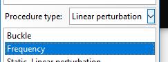
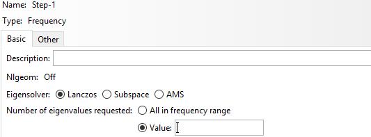
3.      In the Step module, select the ‘Linear Perturbation’ procedure, and select the ‘Frequency’ option. 

4.      In the menu that comes up next, you can specify the maximum frequency of the vibration mode you care about $–$ this is usually the most useful option for real design applications but for homework problems we don’t usually have a reason to look for a particular frequency range so it’s better to specify how many vibration modes you want to look at $–$ for this purpose, check the ‘Value’ radio button and enter a suitable number of vibration modes into the box.   Of course, the more you ask for, the longer the calculation will take.    The higher frequency modes tend to also need a finer mesh.   Usually 30-50 modes is more than enough.

5.     

6.      You can generate a mesh in the usual way.  Note that choice of element type can be important in dynamic simulations; you are likely to see hourglassing in some reduced integration elements; and elements that lock are likely to cause problems.

7.      You can define boundary conditions the usual way in the Load module.   In dynamic simulations, you don’t have to worry about constraining rigid body modes.   You can also use the ‘Predefined Field’ tab in the ‘Load’ module to define initial velocity distributions in your part.   You can’t define initial displacements.   If you need to do this, you will have to run a separate static step just before the explicit dynamic step, and define the initial displacement field as boundary conditions in the static step.

8.      Create the job and run the analysis in the usual way

9.      You can view the natural frequencies and mode shapes in the Visualization module.  The arrows that normally select the increment number are used to step through the modes.   The deformed shape will show the mode shape (you can see the stresses associated with the deformation if you are interested; of course the magnitudes of the stresses are irrelevant, because the amplitude of the mode is arbitrary).   You will see the frequency displayed in the viewport as well.