Chapter 6

 

Equations of Motion, Momentum and Energy for Deformable Solids

 

 

6.1 Linear and angular momentum balance equations for a deformable solid

 

Deformable solids are governed by the same physical laws (Newton’s laws) as a system of particles.   You will hopefully recall that, for a particle system in which particles can only interact by exerting forces on one another (and cannot exert moments on one another):

1.      The net external force acting on the system is equal to the time derivative of the total linear momentum of the system

2.      The total external moment acting on the system is equal to the rate of change of its total angular momentum

3.      The rate of work done by external forces is equal to the sum of the rate of change of kinetic energy of the system and the rate of work done by internal forces.

 

A deformable solid can be thought of as an infinite number of infinitesimal particles.   For a system of this kind, the balance laws can be re-written as a set of partial differential equations, as outlined in the sections to follow.

 

 

6.1.1 Linear momentum balance in terms of Cauchy stress

 

Let ${\sigma }_{ij}$ denote the Cauchy stress distribution within a deformed solid.  Assume that the solid is subjected to a body force $b_i$, and let $u_i,v_i$ and $a_i$ denote the displacement, velocity and acceleration of a material particle at position $y_i$  in the deformed solid.

 

Newton’s third law of motion (F=ma) can be expressed as

${\nabla }_y\cdot \sigma +\rho b=\rho a\text{ or }\frac{\partial {\sigma }_{ij}}{\partial y_i}+\rho b_j=\rho a_j$

Written out in full

$\begin{array}{l}\frac{\partial {\sigma }_{11}}{\partial y_1}+\frac{\partial {\sigma }_{21}}{\partial y_2}+\frac{\partial {\sigma }_{31}}{\partial y_3}+\rho b_1=\rho a_1\\ \frac{\partial {\sigma }_{12}}{\partial y_1}+\frac{\partial {\sigma }_{22}}{\partial y_2}+\frac{\partial {\sigma }_{32}}{\partial y_3}+\rho b_2=\rho a_2\\ \frac{\partial {\sigma }_{13}}{\partial y_1}+\frac{\partial {\sigma }_{23}}{\partial y_2}+\frac{\partial {\sigma }_{33}}{\partial y_3}+\rho b_3=\rho a_3\end{array}$

Note that the derivative is taken with respect to position in the actual, deformed solid. For the special (but rather common) case of a solid in static equilibrium in the absence of body forces

$\frac{\partial {\sigma }_{ij}}{\partial y_i}=0$

 

Derivation: Recall that the resultant force acting on an arbitrary volume of material V within a solid is

$P_i={\displaystyle \underset{A}{\int }{T}_i(n)dA+}{\displaystyle \underset{V}{\int }\rho b_{i}dV}$

where T(n) is the internal traction acting on the surface A with normal n that bounds V.

 

The linear momentum of the volume V is

${\Lambda }_i={\displaystyle \underset{V}{\int }\rho v_i}dV$

where v is the velocity vector of a material particle in the deformed solid. Express T in terms of ${\sigma }_{ij}$ and set $P_i=d{\Lambda }_i/dt$

${\displaystyle \underset{A}{\int }{\sigma }_{ji}{n}_{j}dA+}{\displaystyle \underset{V}{\int }\rho b_{i}dV}=\frac{d}{dt}\left\{{\displaystyle \underset{V}{\int }\rho v_i}dV\right\}$

Apply the divergence theorem to convert the first integral into a volume integral, and note that one can show (see Appendix D) that

$\frac{d}{dt}\left\{{\displaystyle \underset{V}{\int }\rho v_i}dV\right\}={\displaystyle \underset{V}{\int }\rho a_i}dV$

so

${\displaystyle \underset{V}{\int }\frac{\partial {\sigma }_{ji}}{\partial y_j}dV+}{\displaystyle \underset{V}{\int }\rho b_{i}dV}={\displaystyle \underset{V}{\int }\rho a_i}dV\Rightarrow {\displaystyle \underset{V}{\int }\left(\frac{\partial {\sigma }_{ji}}{\partial y_j}+\rho b_i-\rho a_i\right)}dV=0$

Since this must hold for every volume of material within a solid, it follows that

$\frac{\partial {\sigma }_{ji}}{\partial y_j}+\rho b_i=\rho a_i$

as stated.

 

 

6.1.2 Angular momentum balance in terms of Cauchy stress

 

Conservation of angular momentum for a continuum requires that the Cauchy stress satisfy

${\sigma }_{ji}={\sigma }_{ij}$

i.e. the stress tensor must be symmetric.

 

Derivation: write down the equation for balance of angular momentum for the region V within the  deformed solid

${\displaystyle \underset{A}{\int }y\times TdA}+{\displaystyle \underset{V}{\int }y\times \rho bdV}=\frac{d}{dt}\left\{{\displaystyle \underset{V}{\int }y\times \rho vdV}\right\}$

Here, the left hand side is the resultant moment (about the origin) exerted by tractions and body forces acting on a general region within a solid.  The right hand side is the total angular momentum of the solid about the origin.

 

We can write the same expression using index notation

${\displaystyle \underset{A}{\int }{\in }_{ijk}{y}_j{T}_{k}dA}+{\displaystyle \underset{V}{\int }{\in }_{ijk}{y}_j{b}_k\rho dV}=\frac{d}{dt}\left\{{\displaystyle \underset{V}{\int }{\in }_{ijk}{y}_j{v}_k\rho dV}\right\}$

Express T in terms of ${\sigma }_{ij}$ and re-write the first integral as a volume integral using the divergence theorem

$\begin{array}{l}{\displaystyle \underset{A}{\int }{\in }_{ijk}{y}_j{T}_{k}dA}={\displaystyle \underset{A}{\int }{\in }_{ijk}{y}_j{\sigma }_{mk}{n}_{m}dA}={\displaystyle \underset{V}{\int }\frac{\partial }{\partial x_m}\left({\in }_{ijk}{y}_j{\sigma }_{mk}\right)dV}\\ ={\displaystyle \underset{V}{\int }{\in }_{ijk}\left({\delta }_{jm}{\sigma }_{mk}+y_j\frac{\partial {\sigma }_{mk}}{\partial x_m}\right)dV}\end{array}$

We may also show (see Appendix D) that

$\frac{d}{dt}\left\{{\displaystyle \underset{V}{\int }{\in }_{ijk}{y}_j{v}_k\rho dV}\right\}={\displaystyle \underset{V}{\int }{\in }_{ijk}{y}_j{a}_k\rho dV}$

Substitute the last two results into the angular momentum balance equation to see that

$\begin{array}{l}{\displaystyle \underset{V}{\int }{\in }_{ijk}\left({\delta }_{jm}{\sigma }_{mk}+y_j\frac{\partial {\sigma }_{mk}}{\partial x_m}\right)dV}+{\displaystyle \underset{V}{\int }{\in }_{ijk}{y}_j{b}_k\rho dV}={\displaystyle \underset{V}{\int }{\in }_{ijk}{y}_j{a}_k\rho dV}\\ \Rightarrow {\displaystyle \underset{V}{\int }{\in }_{ijk}{\delta }_{jm}{\sigma }_{mk}=-}{\displaystyle \underset{V}{\int }{\in }_{ijk}{y}_j\left(\frac{\partial {\sigma }_{mk}}{\partial y_m}+\rho b_k-\rho a_k\right)dV}\end{array}$

The integral on the right hand side of this expression is zero, because the stresses must satisfy the linear momentum balance equation.  Since this holds for any volume V, we conclude that

$\begin{array}{l}{\in }_{ijk}{\delta }_{jm}{\sigma }_{mk}={\in }_{ijk}{\sigma }_{jk}=0\\ \Rightarrow {\in }_{imn}{\in }_{ijk}{\sigma }_{jk}=0\\ \Rightarrow \left({\delta }_{jm}{\delta }_{kn}-{\delta }_{mk}{\delta }_{nj}\right){\sigma }_{jk}=0\\ \Rightarrow {\sigma }_{mn}-{\sigma }_{nm}=0\end{array}$

which is the result we wanted.

 

 

 

 

 

 

 

 

6.1.3 Equations of motion in terms of other stress measures

 

In terms of nominal and material stress the balance of linear momentum is

$\nabla \cdot S+{\rho }_{0}b={\rho }_{0}a\frac{S_{ij}}{\partial x_i}+{\rho }_0{b}_j={\rho }_0{a}_j$

$\nabla \cdot \left[\Sigma \cdot F^T\right]+{\rho }_{0}b={\rho }_{0}a\frac{\partial \left({\Sigma }_{ik}{F}_{jk}\right)}{\partial x_i}+{\rho }_0{b}_j={\rho }_0{a}_j$

Note that the derivatives are taken with respect to position in the undeformed solid.

 

The angular momentum balance equation is

$⥄⥄⥄⥄⥄⥄⥄⥄F\cdot S={\left[F\cdot S\right]}^T⥄⥄⥄⥄⥄⥄⥄\Sigma ={\Sigma }^{{\rm T}}$

 

 

To derive these results, you can start with the integral form of the linear momentum balance in terms of Cauchy stress

${\displaystyle \underset{A}{\int }{\sigma }_{ji}{n}_{j}dA+}{\displaystyle \underset{V}{\int }\rho b_{i}dV}=\frac{d}{dt}\left\{{\displaystyle \underset{V}{\int }\rho v_i}dV\right\}$

Recall (or see Appendix D for a reminder) that area elements in the deformed and undeformed solids are related through

$dA{n}_i^{}=J{F}_{ki}^{-1}{n}_k^{0}d{A}_0$

In addition, volume elements are related by $dV=Jd{V}_0$.  We can use these results to re-write the integrals as integrals over a volume in the undeformed solid as

${\displaystyle \underset{A0}{\int }{\sigma }_{ji}J{F}_{kj}^{-1}{n}_k^{0}d{A}_0+}{\displaystyle \underset{V0}{\int }\rho b_{i}Jd{V}_0}=\frac{d}{dt}\left\{{\displaystyle \underset{V0}{\int }\rho v_i}Jd{V}_0\right\}$

Finally, recall that $S_{ij}=J{F}_{ik}^{-1}{\sigma }_{kj}$ and that $J\rho ={\rho }_0$ to see that

${\displaystyle \underset{A0}{\int }S{}_{ki}{n}_k^{0}d{A}_0+}{\displaystyle \underset{V0}{\int }\rho {}_0{b}_{i}d{V}_0}=\frac{d}{dt}\left\{{\displaystyle \underset{V0}{\int }\rho {}_0{v}_i}d{V}_0\right\}$

Apply the divergence theorem to the first term and rearrange

${\displaystyle \underset{V}{\int }\left(\frac{\partial S_{ji}}{\partial x_j}+{\rho }_0{b}_i-{\rho }_0\frac{d{v}_i}{dt}\right)}d{V}_0=0$

Once again, since this must hold for any material volume, we conclude that

$\frac{S_{ij}}{\partial x_i}+{\rho }_0{b}_j={\rho }_0{a}_j$

The linear momentum balance equation in terms of material stress follows directly, by substituting into this equation for $S_{ij}$ in terms of ${\Sigma }_{ij}$

 

The angular momentum balance equation can be derived simply by substituting into the momentum balance equation in terms of Cauchy stress ${\sigma }_{ij}={\sigma }_{ji}$

 

 

6.1.4 Equations of motion and equilibrium equations for small deformations

 

The general equations of motion for a deformable solid are hard to solve, because the shape of the solid must be calculated as part of the solution.   In many engineering applications, the deformation is small enough to be neglected.   If this is the case, we can simplify the calculations as follows

 

1. We neglect the differences between the various stress measures described in Section 6.1.3.  
2. We neglect the difference between the density of the deformed and undeformed solid
3. We satisfy the equations of motion (or equilibrium) on the undeformed solid, instead of the deformed solid. 

 

Accordingly, let $x{}_i$ denote the position of a material particle in the undeformed solid, and let ${\rho }_0$ denote the mass density of the undeformed material.   Assume that the solid is subjected to a body force b per unit mass.   Newton’s third law of motion (F=ma) can be expressed as

$\nabla \cdot \sigma +{\rho }_{0}b={\rho }_{0}a\text{ or }\frac{\partial {\sigma }_{ij}}{\partial x_i}+{\rho }_0{b}_j={\rho }_0{a}_j$

Written out in full

$\begin{array}{l}\frac{\partial {\sigma }_{11}}{\partial x_1}+\frac{\partial {\sigma }_{21}}{\partial x_2}+\frac{\partial {\sigma }_{31}}{\partial x_3}+{\rho }_0{b}_1={\rho }_0{a}_1\\ \frac{\partial {\sigma }_{12}}{\partial x_1}+\frac{\partial {\sigma }_{22}}{\partial x_2}+\frac{\partial {\sigma }_{32}}{\partial x_3}+{\rho }_0{b}_2={\rho }_0{a}_2\\ \frac{\partial {\sigma }_{13}}{\partial x_1}+\frac{\partial {\sigma }_{23}}{\partial x_2}+\frac{\partial {\sigma }_{33}}{\partial x_3}+{\rho }_0{b}_3={\rho }_0{a}_3\end{array}$

For the special (but rather common) case of a solid in static equilibrium in the absence of body forces

$\frac{\partial {\sigma }_{ij}}{\partial x_i}=0$

 

 

Example: The stress field

${\sigma }_{ij}=\frac{-3P_k{y}_k{y}_i{y}_j}{4\pi R^5}R=\sqrt{y_k{y}_k}$

represents the stress in an infinite, incompressible linear elastic solid that is subjected to a point force with components $P_k$ acting at the origin (you can visualize a point force as a very large body force which is concentrated in a very small region around the origin).

 

(a)    Verify that the stress field is in static equilibrium

 

This is a tedious exercise in index notation

 

$\frac{\partial {\sigma }_{ij}}{\partial y_i}=-\frac{3P_k}{4\pi }\left(\frac{{\delta }_i{}_k{y}_i{y}_j}{R^5}+\frac{y_k{\delta }_{ii}{y}_j}{R^5}+\frac{y_k{y}_i{\delta }_{ij}}{R^5}-5\frac{y_k{y}_i{y}_j}{R^6}\frac{y_i}{R}\right)=0$

 

 

 

(b)   Consider a spherical region of material centered at the origin.  This region is subjected to (1) the body force acting at the origin; and (2) a force exerted by the stress field on the outer surface of the sphere.   Calculate the resultant force exerted on the outer surface of the sphere by the stress, and show that it is equal in magnitude and opposite in direction to the body force.

 

The traction acting on the exterior surface is $t_i={\sigma }_{ij}{n}_i$ and a unit vector normal vector to a sphere radius R centered at the origin is $n_i=y_i/R$.   The resultant force is thus

$F_j=\frac{-3}{4\pi }{P}_k{\displaystyle \underset{S}{\int }\frac{y_k{y}_j}{R^3}}dA$

The integral clearly vanishes for $k\ne j$ by symmetry.   Choosing k=j=3 without loss of generality we can evaluate the remaining integral in spherical-polar coordinates as

$F_3=\frac{-3}{4\pi }{P}_3{\displaystyle \underset{0}{\overset{2\pi }{\int }}{\displaystyle \underset{0}{\overset{\pi }{\int }}\frac{{\left(R\cos \theta \right)}^2}{R^3}{R}^2\sin \theta d\theta d\varphi }}=-P_3$

 

 

Example Let $\varphi$ be a twice differentiable, scalar function of position.  Derive a plane stress field from $\varphi$ by setting

${\sigma }_{11}=\frac{{\partial }^2\varphi }{\partial y_2^2}{\sigma }_{22}=\frac{{\partial }^2\varphi }{\partial y_1^2}{\sigma }_{12}={\sigma }_{21}=-\frac{{\partial }^2\varphi }{\partial y_1\partial y_2}$

Show that this stress field satisfies the equations of stress equilibrium with zero body force.

 

The equilibrium formulas (with zero body force) are

$\begin{array}{l}\frac{\partial {\sigma }_{11}}{\partial y_1}+\frac{\partial {\sigma }_{21}}{\partial y_2}+\frac{\partial {\sigma }_{31}}{\partial y_3}=0\\ \frac{\partial {\sigma }_{12}}{\partial y_1}+\frac{\partial {\sigma }_{22}}{\partial y_2}+\frac{\partial {\sigma }_{32}}{\partial y_3}=0\\ \frac{\partial {\sigma }_{13}}{\partial y_1}+\frac{\partial {\sigma }_{23}}{\partial y_2}+\frac{\partial {\sigma }_{33}}{\partial y_3}=0\end{array}$

The third equation is satisfied trivially.   The others can be verified by substitution

$\begin{array}{l}\frac{\partial {\sigma }_{11}}{\partial y_1}+\frac{\partial {\sigma }_{21}}{\partial y_2}+\frac{\partial {\sigma }_{31}}{\partial y_3}=\frac{\partial }{\partial y_1}\left(\frac{{\partial }^2\varphi }{\partial y_2^2}\right)+\frac{\partial }{\partial y_2}\left(-\frac{{\partial }^2\varphi }{\partial y_1\partial y_2}\right)=0\\ \frac{\partial {\sigma }_{12}}{\partial y_1}+\frac{\partial {\sigma }_{22}}{\partial y_2}+\frac{\partial {\sigma }_{32}}{\partial y_3}=\frac{\partial }{\partial y_1}\left(-\frac{{\partial }^2\varphi }{\partial y_1\partial y_2}\right)+\frac{\partial }{\partial y_2}\left(\frac{{\partial }^2\varphi }{\partial y_1^2}\right)=0\end{array}$

 

 

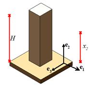
Example: A prismatic concrete column of mass density $\rho$ supports its own weight, as shown below.  (Assume that the solid is subjected to a uniform gravitational body force of magnitude g per unit mass). Show that the stress distribution

${\sigma }_{22}=-\rho g(H-x_2)$

satisfies the equations of static equilibrium

$\frac{\partial {\sigma }_{ij}}{\partial x_i}+\rho b_j=0$

and also satisfies the boundary conditions ${\sigma }_{ij}{n}_i=0$

on all free boundaries.

 

The body force (per unit mass) is $b=-g{e}_2$ .   For this case, the equilibrium equations (written out in full) are

$\begin{array}{l}\frac{\partial {\sigma }_{11}}{\partial y_1}+\frac{\partial {\sigma }_{21}}{\partial y_2}+\frac{\partial {\sigma }_{31}}{\partial y_3}=0\\ \frac{\partial {\sigma }_{12}}{\partial y_1}+\frac{\partial {\sigma }_{22}}{\partial y_2}+\frac{\partial {\sigma }_{32}}{\partial y_3}-\rho g=0\\ \frac{\partial {\sigma }_{13}}{\partial y_1}+\frac{\partial {\sigma }_{23}}{\partial y_2}+\frac{\partial {\sigma }_{33}}{\partial y_3}=0\end{array}$

The first and last equatinos are satisfied automatically, and substituting for the stress into the second and evaluating the derivative shows that that, too, is satisfied.

 

On the sides of the column, the normal vectors point in the $\pm e_1,\pm e_2$  directions.   Since ${\sigma }_{1i}=0,{\sigma }_{3i}=0,{\sigma }_{12}={\sigma }_{32}=0$  it follows that $n_j{\sigma }_{ji}=0$ on the sides.     The stress is zero at $x_2=H$ , so the tractions on the top face are also zero.

 

 

 

6.2 Work done by stresses

 

In this section, we derive formulas that enable you to calculate the work done by stresses acting on a solid. 

 

6.2.1 Work done by Cauchy stresses

 

Consider a solid with mass density ${\rho }_0$ in its initial configuration, and density $\rho$ in the deformed solid. Let ${\sigma }_{ij}$ denote the Cauchy stress distribution within the solid.  Assume that the solid is subjected to a body force $b_i$ (per unit mass), and let $u_i,v_i$ and $a_i$ denote the displacement, velocity and acceleration of a material particle at position $y_i$  in the deformed solid. In addition, let

$D_{ij}=\frac{1}{2}\left(\frac{\partial v_i}{\partial y_j}+\frac{\partial v_j}{\partial y_i}\right)$

denote the stretch rate in the solid.

 

The rate of work done by Cauchy stresses per unit deformed volume is then ${\sigma }_{ij}{D}_{ij}$.  This energy is either dissipated as heat or stored as internal energy in the solid, depending on the material behavior.

 

We shall show that the rate of work done by internal forces acting on any sub-volume V bounded by a surface A in the deformed solid can be calculated from

$\dot{r}={\displaystyle \underset{A}{\int }{T}_i^{(n)}{v}_{i}dA}+{\displaystyle \underset{V}{\int }\rho b_i{v}_{i}dV}={\displaystyle \underset{V}{\int }{\sigma }_{ij}{D}_{ij}dV}+\frac{d}{dt}\left\{{\displaystyle \underset{V}{\int }\frac{1}{2}\rho v_i{v}_{i}dV}\right\}$

Here, the two terms on the left hand side represent the rate of work done by tractions and body forces acting on the solid (work done = force x velocity).  The first term on the right-hand side can be interpreted as the work done by Cauchy stresses; the second term is the rate of change of kinetic energy. 

 

Derivation: Substitute for $T_i^{(n)}$ in terms of Cauchy stress to see that

$\dot{r}={\displaystyle \underset{A}{\int }{T}_i^{(n)}{v}_{i}dA}+{\displaystyle \underset{V}{\int }\rho b_i{v}_{i}dV}={\displaystyle \underset{A}{\int }{n}_j{\sigma }_{ji}{v}_{i}dA}+{\displaystyle \underset{V}{\int }\rho b_i{v}_{i}dV}$

Now, apply the divergence theorem to the first term on the right hand side

$\dot{r}={\displaystyle \underset{V}{\int }\frac{\partial }{\partial y_j}\left({\sigma }_{ji}{v}_i\right)dV}+{\displaystyle \underset{V}{\int }\rho b_i{v}_{i}dV}$

Evaluate the derivative and collect together the terms involving body force and stress divergence

$\dot{r}={\displaystyle \underset{V}{\int }\left\{{\sigma }_{ji}\frac{\partial v_i}{\partial y_j}+\left(\frac{\partial {\sigma }_{ji}}{\partial y_j}+\rho b_i\right)v_i\right\}dV}$

Recall the equation of motion

$\frac{\partial {\sigma }_{ji}}{\partial y_j}+\rho b_i=\rho a_i$

and note that since the stress is symmetric ${\sigma }_{ij}={\sigma }_{ji}$

${\sigma }_{ji}\frac{\partial v_i}{\partial y_j}=\frac{1}{2}\left({\sigma }_{ij}+{\sigma }_{ji}\right)\frac{\partial v_i}{\partial y_j}=\frac{1}{2}{\sigma }_{ij}\left(\frac{\partial v_i}{\partial y_j}+\frac{\partial v_j}{\partial y_i}\right)={\sigma }_{ij}{D}_{ij}$

to see that

$\dot{r}={\displaystyle \underset{V}{\int }\left\{{\sigma }_{ij}{D}_{ij}+\rho a_i{v}_i\right\}dV}$

Finally, note that

$\begin{array}{l}{\displaystyle \underset{V}{\int }\rho a_i{v}_{i}dV}={\displaystyle \underset{V_0}{\int }{\rho }_o\frac{d{v}_i}{dt}{v}_{i}d{V}_0=}{\displaystyle \underset{V_0}{\int }{\rho }_o\frac{1}{2}\frac{d}{dt}\left(v_i{v}_i\right)d{V}_0}\\ =\frac{d}{dt}\left({\displaystyle \underset{V_0}{\int }\frac{1}{2}{\rho }_0\left(v_i{v}_i\right)d{V}_0}\right)=\frac{d}{dt}\left({\displaystyle \underset{V_0}{\int }\frac{1}{2}{\rho }_0\left(v_i{v}_i\right)d{V}_0}\right)=\frac{d}{dt}{\displaystyle \underset{V_{}}{\int }\frac{1}{2}\rho \left(v_i{v}_i\right)dV}\end{array}$

Finally, substitution leads to

$\dot{r}={\displaystyle \underset{A}{\int }{T}_i^{(n)}{v}_{i}dA}+{\displaystyle \underset{V}{\int }\rho b_i{v}_{i}dV}={\displaystyle \underset{V}{\int }{\sigma }_{ij}{D}_{ij}dV}+\frac{d}{dt}\left\{{\displaystyle \underset{V}{\int }\frac{1}{2}\rho v_i{v}_{i}dV}\right\}$

as required.

 

 

 

6.2.2 Rate of mechanical work in terms of other stress measures

 

 The rate of work done per unit undeformed volume by Kirchhoff stress is ${\tau }_{ij}{D}_{ij}$

 The rate of work done per unit undeformed volume by Nominal stress is $S_{ij}{\dot{F}}_{ji}$

 The rate of work done per unit undeformed volume by Material stress is ${\Sigma }_{ij}{\dot{E}}_{ij}$

 

This shows that nominal stress and deformation gradient are work conjugate, as are material stress and Lagrange strain.

 

In addition, the rate of work done on a volume $V_0$ of the undeformed solid can be expressed as

$\dot{r}={\displaystyle \underset{A}{\int }{T}_i^{(n)}{v}_{i}dA}+{\displaystyle \underset{V}{\int }\rho b_i{v}_{i}dV}={\displaystyle \underset{V_0}{\int }{\tau }_{ij}{D}_{ij}d{V}_0}+\frac{d}{dt}\left\{{\displaystyle \underset{V_0}{\int }\frac{1}{2}{\rho }_0{v}_i{v}_{i}d{V}_0}\right\}$

$\dot{r}={\displaystyle \underset{A}{\int }{T}_i^{(n)}{v}_{i}dA}+{\displaystyle \underset{V}{\int }\rho b_i{v}_{i}dV}={\displaystyle \underset{V_0}{\int }{S}_{ij}{\dot{F}}_{ji}d{V}_0}+\frac{d}{dt}\left\{{\displaystyle \underset{V_0}{\int }\frac{1}{2}{\rho }_0{v}_i{v}_{i}d{V}_0}\right\}$

$\dot{r}={\displaystyle \underset{A}{\int }{T}_i^{(n)}{v}_{i}dA}+{\displaystyle \underset{V}{\int }\rho b_i{v}_{i}dV}={\displaystyle \underset{V_0}{\int }{\Sigma }_{ij}{\dot{E}}_{ij}d{V}_0}+\frac{d}{dt}\left\{{\displaystyle \underset{V_0}{\int }\frac{1}{2}{\rho }_0{v}_i{v}_{i}d{V}_0}\right\}$

 

Derivations: The proof of the first result (and the stress power of Kirchhoff stress) is straightforward and is left as an exercise.  To show the second result, note that $T_i^{(n)}dA=n_j^0{S}_{ji}d{A}_0$ and $dV=Jd{V}_0$ to re-write the integrals over the undeformed solid; then and apply the divergence theorem to see that

$\dot{r}={\displaystyle \underset{V_0}{\int }\frac{\partial }{\partial x_j}\left(S_{ji}{v}_i\right)d{V}_0}+{\displaystyle \underset{V0}{\int }\rho b_i{v}_{i}Jd{V}_0}$

Evaluate the derivative, recall that $J\rho ={\rho }_0$ and use the equation of motion

$\frac{S_{ij}}{\partial x_i}+{\rho }_0{b}_j={\rho }_0\frac{d{v}_j}{dt}$

to see that

$\dot{r}={\displaystyle \underset{V_0}{\int }{S}_{ji}\frac{\partial v_i}{\partial x_j}d{V}_0}+{\displaystyle \underset{V0}{\int }{\rho }_0\frac{d{v}_i}{dt}{v}_{i}d{V}_0}$

Finally, note that $\partial v_i/\partial x_j=\left(\partial {\dot{u}}_i/\partial x_j\right)={\dot{F}}_{ij}$ and re-write the second integral as a kinetic energy term as before to obtain the required result.

 

The third result follows by straightforward algebraic manipulations $–$ note that by definition

$S_{ij}{\dot{F}}_{ji}={\Sigma }_{ik}{F}_{jk}^{}{\dot{F}}_{ji}$

Since ${\Sigma }_{ij}$ is symmetric it follows that

${\Sigma }_{ik}{F}_{jk}^{}{\dot{F}}_{ji}=\frac{1}{2}\left({\Sigma }_{ik}+{\Sigma }_{ki}\right)F_{jk}^{}{\dot{F}}_{ji}={\Sigma }_{ik}\frac{1}{2}\left(F_{jk}^{}{\dot{F}}_{ji}+F_{ji}^{}{\dot{F}}_{jk}\right)={\Sigma }_{ik}{\dot{E}}_{ik}$

 

 

6.2.3 Rate of mechanical work for infinitesimal deformations

 

For infintesimal motions all stress measures are equal; and all strain rate measures can be approximated by the infinitesimal strain tensor $\epsilon$.  The rate of work done by stresses per unit volume of either deformed or undeformed solid (the difference is neglected) can be expressed as ${\sigma }_{ij}{\dot{\epsilon }}_{ij}$, and the work done on a volume $V_0$ of the solid is

$\dot{r}={\displaystyle \underset{A}{\int }{T}_i^{(n)}{v}_{i}dA}+{\displaystyle \underset{V}{\int }\rho b_i{v}_{i}dV}={\displaystyle \underset{V_0}{\int }{\sigma }_{ij}{\dot{\epsilon }}_{ij}d{V}_0}+\frac{d}{dt}\left\{{\displaystyle \underset{V_0}{\int }\frac{1}{2}{\rho }_0{v}_i{v}_{i}d{V}_0}\right\}$

 

 

 

6.3 The principle of Virtual Work

 

The principle of virtual work is an alternative way of expressing the equations of motion and equilibrium derived in Section 6.1.  At first sight it appears to be fairly useless, but it turns out to be an extremely useful way of deriving equilibrium equations or equations of motion for a solid in which the deformation is approximated in some way $–$ for example, in a beam, plate or shell.  In addition, the principle of virtual work is also used as the starting point for finite element analysis for nonlinear solids, and so is a particularly important result.

Some definitions are needed before the principle can be stated.  Suppose that a deformable solid is subjected to loading that induces a displacement field $u(x)$, and a velocity field $v(x)$.  The loading consists of a prescribed displacement on part of the boundary (denoted by $S_1$ ), together with a traction t (which may be zero in places) applied to the rest of the boundary (denoted by $S_2$ ).  The loading induces a Cauchy stress ${\sigma }_{ij}$.  The stress field satisfies the angular momentum balance equation ${\sigma }_{ij}={\sigma }_{ji}$.

 

The principle of virtual work is a different way of re-writing partial differential equation for linear moment balance

$\frac{\partial {\sigma }_{ji}}{\partial y_j}+\rho b_i=\rho \frac{d{v}_i}{dt}$

in an equivalent integral form, which is much better suited for computer solution.

 

To express the principle, we define a kinematically admissible virtual velocity field $\delta v(y)$, satisfying  $\delta v=0$ on $S_1$.  You can visualize this field as a small change in the velocity of the solid, if you like, but it is really just an arbitrary differentiable vector field.  The term `kinematically admissible’ is just a complicated way of saying that the field is continuous, differentiable, and satisfies $\delta v=0$ on $S_1$ - that is to say, if you perturb the velocity by $\delta v(y)$, the boundary conditions on displacement are still satisfied.

 

In addition, we define an associated virtual velocity gradient, and virtual stretch rate as

$\delta L_{ij}=\frac{\partial \delta v_i}{\partial y_j}\delta D_{ij}=\frac{1}{2}\left(\frac{\partial \delta v_i}{\partial y_j}+\frac{\partial \delta v_j}{\partial y_i}\right)$

 

The principal of virtual work may be stated in two ways.

 

6.3.1 First version of the principle of virtual work

 

The first is not very interesting, but we will state it anyway.  Suppose that the Cauchy stress satisfies:

1.      The boundary condition $n_i{\sigma }_{ij}=t_j$ on $S_2$

2.      The linear momentum balance equation

$\frac{\partial {\sigma }_{ji}}{\partial y_j}+\rho b_i=\rho \frac{d{v}_i}{dt}$

Then the virtual work equation

${\displaystyle \underset{V}{\int }\sigma :\delta DdV+{\displaystyle \underset{V}{\int }\rho \frac{dv}{dt}\cdot \delta vdV}-{\displaystyle \underset{V}{\int }\rho b\cdot \delta vdV}}-{\displaystyle \underset{S}{\int }t\cdot \delta v}dA=0$

Or equivalently, with index notation

${\displaystyle \underset{V}{\int }{\sigma }_{ij}\delta D_{ij}dV+{\displaystyle \underset{V}{\int }\rho \frac{d{v}_i}{dt}\delta v_i}dV-{\displaystyle \underset{V}{\int }\rho b_i\delta v_{i}dV-{\displaystyle \underset{S_2}{\int }{t}_i\delta v_i}}}dA=0$

is satisfied for all virtual velocity fields.

 

Proof:  Observe that since the Cauchy stress is symmetric

${\sigma }_{ij}\delta D_{ij}=\frac{1}{2}{\sigma }_{ij}\left(\frac{\partial \delta v_i}{\partial y_j}+\frac{\partial \delta v_j}{\partial y_i}\right)=\frac{1}{2}\left({\sigma }_{ji}\frac{\partial \delta v_i}{\partial y_j}+{\sigma }_{ij}\frac{\partial \delta v_j}{\partial y_i}\right)={\sigma }_{ji}\frac{\partial \delta v_i}{\partial y_j}$

Next, note that

${\sigma }_{ji}\frac{\partial v_i}{\partial y_j}=\frac{\partial }{\partial y_j}\left({\sigma }_{ji}\delta v_i\right)-\frac{\partial {\sigma }_{ji}}{\partial y_j}\delta v_i$

Finally, substituting the latter identity into the virtual work equation, applying the divergence theorem, using the linear momentum balance equation and boundary conditions on $\sigma$ and $\delta v(y)$ we obtain the required result.

 

6.3.2 Second version of the principle of virtual work

 

The converse of this statement is much more interesting and useful.  Suppose that ${\sigma }_{ij}$ satisfies the virtual work equation

${\displaystyle \underset{V}{\int }\sigma :\delta DdV+{\displaystyle \underset{V}{\int }\rho \frac{dv}{dt}\cdot \delta vdV}-{\displaystyle \underset{V}{\int }\rho b\cdot \delta vdV}}-{\displaystyle \underset{S}{\int }t\cdot \delta v}dA=0$

Or, using index notation

${\displaystyle \underset{V}{\int }{\sigma }_{ij}\delta D_{ij}dV+{\displaystyle \underset{V}{\int }\rho \frac{d{v}_i}{dt}\delta v_i}dV-{\displaystyle \underset{V}{\int }\rho b_i\delta v_{i}dV-{\displaystyle \underset{S_2}{\int }{t}_i\delta v_i}}}dA=0$

for all virtual velocity fields $\delta v(y)$.  Then the stress field must satisfy

3.      The boundary condition $n_i{\sigma }_{ij}=t_j$ on $S_2$

4.      The linear momentum balance equation

$\frac{\partial {\sigma }_{ji}}{\partial y_j}+\rho b_i=\rho \frac{d{v}_i}{dt}$

The significance of this result is that it gives us an alternative way to solve for a stress field that satisfies the linear momentum balance equation, which avoids having to differentiate the stress.  It is not easy to differentiate functions accurately in the computer, but it is easy to integrate them.  The virtual work statement is the starting point for any finite element solution involving deformable solids.

 

 

Proof: Follow the same preliminary steps as before, i..e.

${\sigma }_{ij}\delta D_{ij}=\frac{1}{2}{\sigma }_{ij}\left(\frac{\partial \delta v_i}{\partial y_j}+\frac{\partial \delta v_j}{\partial y_i}\right)=\frac{1}{2}\left({\sigma }_{ji}\frac{\partial \delta v_i}{\partial y_j}+{\sigma }_{ij}\frac{\partial \delta v_j}{\partial y_i}\right)={\sigma }_{ji}\frac{\partial \delta v_i}{\partial y_j}$

${\sigma }_{ji}\frac{\partial v_i}{\partial y_j}=\frac{\partial }{\partial y_j}\left({\sigma }_{ji}\delta v_i\right)-\frac{\partial {\sigma }_{ji}}{\partial y_j}\delta v_i$

and substitute into the virtual work equation

${\displaystyle \underset{V}{\int }\left\{\frac{\partial }{\partial y_j}\left({\sigma }_{ji}\delta v_i\right)-\frac{\partial {\sigma }_{ji}}{\partial y_j}\delta v_i\right\}dV+{\displaystyle \underset{V}{\int }\rho \frac{d{v}_i}{dt}\delta v_i}dV-{\displaystyle \underset{V}{\int }\rho b_i\delta v_{i}dV-{\displaystyle \underset{S_2}{\int }{t}_i\delta v_i}}}dA=0$

Apply the divergence theorem to the first term in the first integral, and recall that $\delta v=0$ on $S_1$, we see that

$-{\displaystyle \underset{V}{\int }\left\{\frac{\partial {\sigma }_{ji}}{\partial y_j}+\rho b_i-\rho \frac{d{v}_i}{dt}\right\}\delta v_{i}dV}+{\displaystyle \underset{S_2}{\int }\left({\sigma }_{ji}{n}_j-t_i\right)\delta v_i}dA=0$

Since this must hold for all virtual velocity fields we could choose

$\delta v_i=f(y)\left\{\frac{\partial {\sigma }_{ji}}{\partial y_j}+\rho b_i-\rho \frac{d{v}_i}{dt}\right\}$

where $f(y)=0$ is an arbitrary function that is positive everywhere inside the solid, but is equal to zero on $S$.  For this choice, the virtual work equation reduces to

$-{\displaystyle \underset{V}{\int }f\left(y\right)\left\{\frac{\partial {\sigma }_{ji}}{\partial y_j}+\rho b_i-\rho \frac{d{v}_i}{dt}\right\}\left\{\frac{\partial {\sigma }_{ki}}{\partial y_k}+\rho b_i-\rho \frac{d{v}_i}{dt}\right\}dV}=0$

and since the integrand is positive everywhere the only way the equation can be satisfied is if

$\frac{\partial {\sigma }_{ji}}{\partial y_j}+\rho b_i=\rho \frac{d{v}_i}{dt}$

Given this, we can next choose a virtual velocity field that satisfies

$\delta v_i=\left({\sigma }_{ji}{n}_j-t_i\right)$

on $S_2$.  For this choice (and noting that the volume integral is zero) the virtual work equation reduces to

$+{\displaystyle \underset{S_2}{\int }\left({\sigma }_{ji}{n}_j-t_i\right)\left({\sigma }_{ki}{n}_k-t_i\right)}dA=0$

Again, the integrand is positive everywhere (it is a perfect square) and so can vanish only if

${\sigma }_{ji}{n}_j=t_i$

as stated.

 

6.3.3 The Virtual Work equation in terms of other stress measures.

 

It is often convenient to implement the virtual work equation in a finite element code using different stress measures. 

 

To do so, we define

1.      The actual deformation gradient in the solid $F_{ij}={\delta }_{ij}+\frac{\partial u_i}{\partial x_j}$

2.      The virtual rate of change of deformation gradient  $\delta {\dot{F}}_{ij}=\frac{\partial \delta v_i}{\partial y_k}{F}_{kj}=\frac{\partial \delta v_i}{\partial x_j}$

3.      The virtual rate of change of Lagrange strain $\delta {\dot{E}}_{ij}=\frac{1}{2}\left(F_{ki}\delta {\dot{F}}_{kj}+\delta {\dot{F}}_{ki}{F}_{kj}\right)$

In addition, we define (in the usual way)

1.      Kirchhoff stress  ${\tau }_{ij}=J{\sigma }_{ij}$

2.      Nominal (First Piola-Kirchhoff) stress  $S_{ij}=J{F}_{ik}^{-1}{\sigma }_{kj}$

3.      Material (Second Piola-Kirchhoff) stress  ${\Sigma }_{ij}=J{F}_{ik}^{-1}{\sigma }_{kl}{F}_{jl}^{-1}$

 

In terms of these quantities, the virtual work equation may be expressed as

${\displaystyle \underset{V0}{\int }{\tau }_{ij}\delta D_{ij}d{V}_0+{\displaystyle \underset{V_0}{\int }{\rho }_0\frac{d{v}_i}{dt}\delta v_i}d{V}_0-{\displaystyle \underset{V0}{\int }{\rho }_0{b}_i\delta v_{i}d{V}_0-{\displaystyle \underset{S_2}{\int }{t}_i\delta v_i}}}dA=0$

${\displaystyle \underset{V0}{\int }{S}_{ij}\delta {\dot{F}}_{ji}d{V}_0+{\displaystyle \underset{V_0}{\int }{\rho }_0\frac{d{v}_i}{dt}\delta v_i}d{V}_0-{\displaystyle \underset{V0}{\int }{\rho }_0{b}_i\delta v_{i}d{V}_0-{\displaystyle \underset{S_2}{\int }{t}_i\delta v_i}}}dA=0$

${\displaystyle \underset{V0}{\int }{\Sigma }_{ij}\delta {\dot{E}}_{ij}d{V}_0+{\displaystyle \underset{V_0}{\int }{\rho }_0\frac{d{v}_i}{dt}\delta v_i}d{V}_0-{\displaystyle \underset{V0}{\int }{\rho }_0{b}_i\delta v_{i}d{V}_0-{\displaystyle \underset{S_2}{\int }{t}_i\delta v_i}}}dA=0$

Note that all the volume integrals are now taken over the undeformed solid $–$ this is convenient for computer applications, because the shape of the undeformed solid is known.  The area integral is evaluated over the deformed solid, unfortunately.  It can be expressed as an equivalent integral over the undeformed solid, but the result is messy and will be deferred until we actually need to do it.

 

 

6.3.4 The Virtual Work equation for infinitesimal deformations.

 

For infintesimal motions, the Cauchy, Nominal, and Material stress tensors are equal; and the virtual stretch rate can be replaced by the virtual infinitesimal strain rate

$\delta {\dot{\epsilon }}_{ij}=\frac{1}{2}\left(\frac{\partial \delta v_i}{\partial x_j}+\frac{\partial \delta v_j}{\partial x_i}\right)$

There is no need to distinguish between the volume or surface area of the deformed and undeformed solid.  The virtual work equation can thus be expressed as

${\displaystyle \underset{V0}{\int }{\sigma }_{ij}\delta {\dot{\epsilon }}_{ij}d{V}_0+{\displaystyle \underset{V_0}{\int }{\rho }_0\frac{d{v}_i}{dt}\delta v_i}d{V}_0-{\displaystyle \underset{V0}{\int }{\rho }_0{b}_i\delta v_{i}d{V}_0-{\displaystyle \underset{S_2}{\int }{t}_i\delta v_i}}}d{A}_0=0$

for all kinematically admissible velocity fields.

 

 

As a special case, this expression can be applied to a quasi-static state with $v_i=0$. Then, for a stress state ${\sigma }_{ij}$ satisfying the static equilibrium equation ${\sigma }_{ij}/d{x}_i+{\rho }_0{b}_j=0$ and boundary conditions ${\sigma }_{ij}{n}_j=t_i$ on $S_2$, the virtual work equation reduces to

${\displaystyle \underset{V0}{\int }{\sigma }_{ij}\delta {\epsilon }_{ij}d{V}_0}={\displaystyle \underset{V0}{\int }{\rho }_0{b}_i\delta u_{i}d{V}_0+{\displaystyle \underset{S_2}{\int }{t}_i\delta u_{i}dA}}$

In which $\delta u_i$ are kinematically admissible displacements components $(\delta u_i=0$ on S₂) and $\delta {\epsilon }_{ij}=\left(\partial \delta u_i/x_j+\partial \delta u_j/x_i\right)/2$.

 

Conversely, if  the stress state ${\sigma }_{ij}$ satisfies ${\displaystyle \underset{V0}{\int }{\sigma }_{ij}\delta {\epsilon }_{ij}d{V}_0}={\displaystyle \underset{V0}{\int }{\rho }_0{b}_i\delta u_{i}d{V}_0+{\displaystyle \underset{S_2}{\int }{t}_i\delta u_{i}dA}}$ for every set of kinematically admissible virtual displacements, then the stress state ${\sigma }_{ij}$ satisfies the static equilibrium equation ${\sigma }_{ij}/d{x}_i+{\rho }_0{b}_j=0$ and boundary conditions ${\sigma }_{ij}{n}_j=t_i$ on $S_2$. 

 

Example: The shell shown in the figure is subjected to a radial body force $b=\rho b(R)e_R$, and a radial pressure $p_a,p_b$ acting on the surfaces at $R=a$ and $R=b$. The loading induces a spherically symmetric state of stress in the shell, which can be expressed in terms of its components in a spherical-polar coordinate system as ${\sigma }_{RR}{e}_R\otimes e_R+{\sigma }_{\theta \theta }{e}_{\theta }\otimes e_{\theta }+{\sigma }_{\varphi \varphi }{e}_{\varphi }\otimes e_{\varphi }$ (or if you prefer matrix notation

$\sigma =\left[\begin{array}{ccc}{\sigma }_{RR}& 0& 0\\ 0& {\sigma }_{\theta \theta }& 0\\ 0& 0& {\sigma }_{\varphi \varphi }\end{array}\right]$

 

(a) By considering a virtual velocity of the form $\delta v=w(R)e_R$, (i.e. all points in the sphere can only move in the radial direction, but they can move by an arbitrary displacement) show that the stress state is in static equilibrium if

 

${\displaystyle \underset{a}{\overset{b}{\int }}\left\{{\sigma }_{RR}\frac{dw}{dR}+\left({\sigma }_{\theta \theta }+{\sigma }_{\varphi \varphi }\right)\frac{w}{R}\right\}4\pi R^{2}dR}-{\displaystyle \underset{a}{\overset{b}{\int }}b(R)w(R)4\pi R^{2}dR-4\pi a^2{p}_{a}w(a)+}4\pi b^2{p}_{b}w(b)=0$

for all w(R). 

 

 

(b) Hence, show that the stress state must satisfy

$\frac{d{\sigma }_{RR}}{dR}+\frac{1}{R}\left(2{\sigma }_{RR}-{\sigma }_{\theta \theta }-{\sigma }_{\varphi \varphi }\right)+b=0{\sigma }_{RR}=-p_a\left(R=a\right){\sigma }_{RR}=-p_b\left(R=b\right)$

 

 

The principle of virtual work will usually magically give you a simplified form of the general equilibrium equation for any simplified kind of deformation.   There is a standard process to follow, which involves two steps: (i) substitute a virtual displacement field that has the same form as the simplified kind of motion; and then (usually) (ii) integrate the virtual work equation by parts to remove any derivatives of the displacement field.  

 

We will use this method here.   To evaluate the virtual work equation, we must first calculate the virtual stretch rate $\delta D$.  By definition $D=\left\{\nabla v+{\left(\nabla v\right)}^T\right\}/2$ .   We can use the formula from Section 3.5.8 to calculate the gradient in spherical polar coordinates

$\nabla v\equiv \left[\begin{array}{ccc}\frac{\partial v_R}{\partial R}& \frac{1}{R}\frac{\partial v_R}{\partial \theta }-\frac{v_{\theta }}{R}& \frac{1}{R\sin \theta }\frac{\partial v_R}{\partial \varphi }-\frac{v_{\varphi }}{R}\\ \frac{\partial v_{\theta }}{\partial R}& \frac{1}{R}\frac{\partial v_{\theta }}{\partial \theta }+\frac{v_R}{R}& \frac{1}{R\sin \theta }\frac{\partial v_{\theta }}{\partial \varphi }-\cot \theta \frac{v_{\varphi }}{R}\\ \frac{\partial v_{\varphi }}{\partial R}& \frac{1}{R}\frac{\partial v_{\varphi }}{\partial \theta }& \frac{1}{R\sin \theta }\frac{\partial v_{\varphi }}{\partial \varphi }+\cot \theta \frac{v_{\theta }}{R}+\frac{v_R}{R}\end{array}\right]=\left[\begin{array}{ccc}\frac{dw}{dR}& 0& 0\\ 0& \frac{w}{R}& 0\\ 0& 0& \frac{w}{R}\end{array}\right]$

 

This is symmetric already, so $D=\nabla v$ in this case.   It follows that

$\sigma :\delta D={\sigma }_{RR}\frac{dw}{dR}+\left({\sigma }_{\theta \theta }+{\sigma }_{\varphi \varphi }\right)\frac{w}{R}$

 

The remaining terms in the virtual work equation are standard dot products, and the volume integral can be re-written as an integral with respect to the radial coordinate R, so the virtual work principle therefore reduces to

$\begin{array}{l}{\displaystyle \underset{V}{\int }\sigma :\delta DdV-{\displaystyle \underset{V}{\int }\rho b\cdot \delta vdV-{\displaystyle \underset{S}{\int }{t}^{*}\cdot \delta v}dA}}=\\ {\displaystyle \underset{a}{\overset{b}{\int }}\left\{{\sigma }_{RR}\frac{dw}{dR}+\left({\sigma }_{\theta \theta }+{\sigma }_{\varphi \varphi }\right)\frac{w}{R}\right\}4\pi R^{2}dR}-{\displaystyle \underset{a}{\overset{b}{\int }}b(R)w(R)4\pi R^{2}dR-4\pi a^2{p}_{a}w(a)+}4\pi b^2{p}_{b}w(b)=0\end{array}$

 

In this form, the equation does not tell us anything interesting.   However, if we integrate the first term by parts, we can re-write the virtual work equation as

$\begin{array}{l}{\displaystyle \underset{a}{\overset{b}{\int }}\left\{\frac{1}{R^2}\frac{d(R^2{\sigma }_{RR})}{dR}+\left({\sigma }_{\theta \theta }+{\sigma }_{\varphi \varphi }\right)\frac{1}{R}-b(R)\right\}w4\pi R^{2}dR}\\ -4\pi a^2({\sigma }_{RR}(a)+p_a)w(a)+4\pi b^2({\sigma }_{RR}(b)+p_b)w(b)=0\end{array}$

This must vanish for all w.   Since this includes any w with w=0 at R=a,R=B, it follows that

${\displaystyle \underset{a}{\overset{b}{\int }}\left\{\frac{1}{R^2}\frac{d(R^2{\sigma }_{RR})}{dR}+\left({\sigma }_{\theta \theta }+{\sigma }_{\varphi \varphi }\right)\frac{1}{R}-b(R)\right\}w4\pi R^{2}dR}=0$

This must vanish even if we happen to pick

$w=\frac{1}{R^2}\frac{d(R^2{\sigma }_{RR})}{dR}+\left({\sigma }_{\theta \theta }+{\sigma }_{\varphi \varphi }\right)\frac{1}{R}-b(R)$

which requires that

${\displaystyle \underset{a}{\overset{b}{\int }}{\left\{\frac{1}{R^2}\frac{d(R^2{\sigma }_{RR})}{dR}+\left({\sigma }_{\theta \theta }+{\sigma }_{\varphi \varphi }\right)\frac{1}{R}-b(R)\right\}}^{2}4\pi R^{2}dR}=0$

The integrand is now positive or zero everywhere, so the integral can only be zero if the integrand is zero.   Therefore

$\frac{d{\sigma }_{RR}}{dR}+\frac{1}{R}\left(2{\sigma }_{RR}-{\sigma }_{\theta \theta }-{\sigma }_{\varphi \varphi }\right)+b=0$

Since the integrand vanishes, we now are left with

$-4\pi a^2({\sigma }_{RR}(a)+p_a)w(a)+4\pi b^2({\sigma }_{RR}(b)+p_b)w(b)=0$

Again, this condition must be satisfied for all w, which is only possible if

${\sigma }_{RR}=-p_a\left(R=a\right){\sigma }_{RR}=-p_b\left(R=b\right)$