Chapter 8

 

Small Strain Static Solutions for Elastic Solids

 

In many engineering applications, the component or solid of interest is stiff, and is subjected only to modest stresses.   This is because large stresses, and large shape changes, usually cause a component to fail.  Stiff solids subjected to modest loads experience only small changes in shape, and the material can be assumed to deform elastically.    Under these conditions, it is often possible to calculate exactly the distributions of stress and strain in the solid.   Analysis of this kind is called ‘linear elasticity.’

 

In this chapter, we present a very brief survey of the field of linear elasticity.  Specifically,

1.      We will outline some important general features of solutions to for linear elastic solids subjected to external forces;

2.      We will discuss some solution techniques and present solutions to a few selected problems of interest;

3.      We will discuss energy methods for solving problems involving linear elastic solids.   These will later be used to develop the finite element method for calculating stresses in elastic solids.

 

 

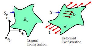
8.1 Summary of the governing equations of linear elasticity

 

For a stiff solid subjected to modest stresses, we can assume

1.      All displacements are small.  This means that we can use the infinitesimal strain tensor to characterize deformation; we do not need to distinguish between stress measures, and we do not need to distinguish between deformed and undeformed configurations of the solid when writing equilibrium equations and boundary conditions.

2.      The material is a linear elastic solid.  In most practical applications, we can also assume the material is isotropic, with Young’s modulus E and Poisson’s ratio $\nu$, and mass density ${\rho }_0$. 

 

In any application, we must be given:

1.      The shape of the solid in its unloaded condition $R$

2.      The initial stress field in the solid (we will take this to be zero)

3.      The elastic constants for the solid $C_{ijkl}$ and its mass density ${\rho }_0$

4.      The thermal expansion coefficients for the solid, and temperature change from the initial configuration $\Delta T$

5.      A body force distribution $b$ (per unit mass) acting on the solid

6.      Boundary conditions, specifying displacements $u^{*}(x)$ on a portion ${\partial }_{1}R$ or tractions on a portion ${\partial }_{2}R$ of the boundary of R

 

Our goal is then to calculate the displacement field $u_i$, the strain field ${\epsilon }_{ij}$ and the stress field ${\sigma }_{ij}$ satisfying the following equations:

 Displacement$—$strain relation $\epsilon =\frac{1}{2}\left(\nabla u+{\left(\nabla u\right)}^T\right)$   or ${\epsilon }_{ij}=\frac{1}{2}\left(\frac{\partial u_i}{\partial x_j}+\frac{\partial u_j}{\partial x_i}\right)$

 The Stress$—$strain-temperature relation $\sigma =C(\epsilon -\alpha \Delta T)$

or, for an isotropic material: ${\sigma }_{ij}=\frac{E}{1+\nu }\left\{{\epsilon }_{ij}+\frac{\nu }{1-2\nu }{\epsilon }_{kk}{\delta }_{ij}\right\}-\frac{E\alpha \Delta T}{1-2\nu }{\delta }_{ij}$

 Equilibrium Equation $\nabla \cdot \sigma +{\rho }_{0}b=0$ or $\frac{\partial {\sigma }_{ij}}{\partial x_i}+{\rho }_0{b}_j=0$ 

 Traction boundary conditions $n\cdot \sigma =t^{*}\text{on}{\partial }_{2}R$ on parts of the boundary where tractions are known.

 

 Displacement boundary conditions $u=u^{*}\text{on}{\partial }_{1}R$  on parts of the boundary where displacements are known.

 

Before actually solving these equations, we will discuss some general features of the solutions.

 

 

8.2 Superposition and linearity of solutions

 

The governing equations of elasticity are linear.  This has two important consequences:

1.      The stresses, strains and displacements in a solid are directly proportional to the loads (or displacements) applied to the solid. 

2.      If you can find two sets of displacements, strains and stresses that satisfy the governing equations, you can add them to create more solutions.

 

These principles can be illustrated clearly using some of the simple solutions derived in the next section.  For example, examine the solution to the pressurized sphere (Sect 4.1.4).    As an example, the radial stress induced by pressure $p_a$ on the interior, and zero pressure on the exterior surface is

${\sigma }_{rr}=\frac{\left(p_a{a}^3\right)}{\left(b^3-a^3\right)}\left(1-\frac{b^3}{r^2}\right)$    

The radial stress induced by pressure $p_b$ on the exterior surface, with zero pressure on the interior surface is

${\sigma }_{rr}=-\frac{p_b{b}^3}{\left(b^3-a^3\right)}\left(1-\frac{a^3}{r^3}\right)$

Note that in both cases the stress is directly proportional to the pressure.  In addition, to find the radial stress by combined pressures $p_a$ on the interior and $p_b$ on the exterior surface, you can just add these two solutions.

 

 

8.3  Uniqueness and existence of solutions to the linear elasticity equations

 

The following results are useful:

1.      If only displacements are prescribed on the boundary of the solid, the governing equations of linear elasticity always have a solution, and the solution is unique.

2.      If mixed boundary conditions are specified, a static solution exists and is unique if the displacements constrain rigid motions. A dynamic solution always exists and is unique, provided the velocity field and displacement field at time t=0 are known.

3.      If only tractions are prescribed on the boundary, a static solution exists only if the tractions are in equilibrium.  In this case, the stresses and strains are unique, but the displacements are not.  A dynamic solution always exists and is unique, again, providing initial conditions are known.

 

 

8.4 Saint-Venant’s principle

 

Saint-Venant’s principle is often invoked to justify approximate solutions to boundary value problems in linear elasticity.  For example, when we solve problems involving bending or axial deformation of slender beams and rods in elementary strength of materials courses, we only specify the resultant forces acting on the ends of a rod, or the magnitudes of point forces acting on a beam, we don’t specify the distribution of traction in detail.  We rely on Saint Venant’s principle to justify this approach. In this context, the principle states the following.

 

The stresses, strains and displacements far from the ends of a rod or beam subjected to end loading depend only on the resultant forces and moments acting on its ends, and do not depend on how the tractions themselves are distributed.

 

Although SVP is widely used, it turns out to be remarkably difficult to prove mathematically.   The difficulty is partly that it is not easy to state the principle itself precisely enough to apply any mathematical machinery to it.  A rigorous statement is given by Sternberg (Q. J. Appl. Mech 11 p. 393 1954), among several other versions.  Here, we will just illustrate the most common applications of the principle through specific examples.

 

One version of SVP can be stated as follows.

 

Suppose that we calculate the stress, strain and displacement induced in a solid by two different traction distributions $t^{(1)}$ and $t^{(2)}$ that act on some small region of a solid with characteristic size a.  If the tractions exert the same resultant force and moment, then the stresses, strains and displacements induced by the two traction distributions at a distance r from the loaded region are identical for large $r/a$. 

 

In practice `large’ usually means $r/a>3$.

 

This principle can be illustrated using a simple example.

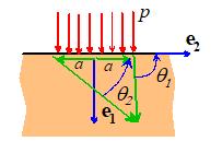
Consider a large solid with a flat surface, as shown in the picture.  It is possible to calculate formulas for the stresses and displacements induced by various pressure distributions acting on the flat surface $–$ the procedure to do this will be outlined later.  For now, we will compare the stresses induced by

1.      A uniform pressure $p(r)=P/\left(\pi a^2\right)r\le a$

2.      A parabolic pressure  $p(r)=\frac{3P}{2\pi ⥄a^2}{(1-r^2/a^2)}^{1/2}r\le a$

You can verify for yourself that both pressure distributions exert a resultant force P acting in the vertical direction on the surface, and exert zero moment about the origin.  The variation of stress down the axis of symmetry ( $r=\sqrt{x_1^2+x_2^2}=0$ ), expressed in cylindrical-polar coordinates, can be derived as

 

 

Case 1: Uniform pressure

${\sigma }_{zz}=-\frac{P}{\pi a^2}\left(1-\frac{z_{}^3}{{(a^2+z^2)}^{3/2}}\right){\sigma }_{rr}={\sigma }_{\theta \theta }=-\frac{P}{\pi a^2}\left(\frac{1+2\nu }{2}-\frac{(1+\nu )z}{{(a^2+z^2)}^{1/2}}+\frac{z^3}{2{(a^2+z^2)}^{3/2}}\right)$

Case 2: Parabolic pressure

${\sigma }_{zz}=-\frac{3P}{2\pi a^2}\frac{a^2}{\left(a^2+z^2\right)}{\sigma }_{rr}={\sigma }_{\theta \theta }=-\frac{3P}{2\pi a^2}\left\{(1+\nu )\left(1-\frac{z}{a}{\text{tan}}^{\text{-1}}\frac{a}{z}\right)-\frac{1}{2}\frac{a^2}{a^2+z^2}\right\}$

Now, to demonstrate SVP, we want to show that the stresses are equal for large z/a.  We can do this graphically $–$ the figures below compare the variation of vertical and radial stress down the axis of symmetry with z/a.

                      

 

The stresses induced by the two different pressures are clearly indistinguishable for $z/a>3$.  This example helps to quantify what we mean by a `large’ distance.

 

The second commonly used application of SVP is a rather vague statement that

 

 A localized geometrical feature with characteristic size R in a large solid only influences the stress in a region with size approximately 3R surrounding the feature.

 

This is more a rule of thumb than a precise mathematical statement.  It can be illustrated by looking at specific solutions.  For example, the figure below shows the Mises stress contours surrounding a circular hole in a thin rectangular plate that is subjected to extensional loading (calculated using the finite element method). Far from the hole, the stress is uniform.  The contours deviate from the uniform solution in a region that is about three times the hole radius.

 

 

 

 

8.5 Simplified equations for spherically symmetric linear elasticity problems

 

It is easiest to solve the linear elasticity problems if the solid of interest has symmetry of some kind, and is subjected to simple loading.   Spheres and cylinders are two examples.

 

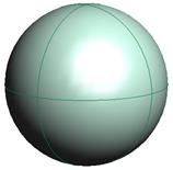
A representative spherically symmetric problem is illustrated in the picture.  We consider a hollow, spherical solid, which is subjected to spherically symmetric loading (i.e. internal body forces, as well as tractions or displacements applied to the surface, are independent of $\theta$ and $\varphi$, and act in the radial direction only).  If the temperature of the sphere is non-uniform, it must also be spherically symmetric (a function of R only).

 

The solution is most conveniently expressed using a spherical-polar coordinate system, illustrated in the figure.  The general procedure for solving problems using spherical and cylindrical coordinates is complicated, and is discussed in detail in Appendix E.  In this section, we summarize the special form of these equations for spherically symmetric problems.

 

As usual, a point in the solid is identified by its spherical-polar co-ordinates $(R,\theta ,\varphi )$. All vectors and tensors are expressed as components in the basis $\left\{e_R,e_{\theta },e_{\varphi }\right\}$ shown in the figure.  For a spherically symmetric problem

 Position Vector       $x=R{e}_R$

 Displacement vector $u=u(R)e_R$

 Body force vector $b={\rho }_{0}b(R)e_R$

 

Here, $u\left(R\right)$ and $b\left(R\right)$ are scalar functions. The stress and strain tensors (written as components in $\{e_R,e_{\theta },e_{\varphi }\}$ ) have the form

$\sigma \equiv \left[\begin{array}{ccc}{\sigma }_{RR}& 0& 0\\ 0& {\sigma }_{\theta \theta }& 0\\ 0& 0& {\sigma }_{\varphi \varphi }\end{array}\right]\epsilon \equiv \left[\begin{array}{ccc}{\epsilon }_{RR}& 0& 0\\ 0& {\epsilon }_{\theta \theta }& 0\\ 0& 0& {\epsilon }_{\varphi \varphi }\end{array}\right]$

and furthermore must satisfy ${\sigma }_{\theta \theta }={\sigma }_{\varphi \varphi }$ ${\epsilon }_{\theta \theta }={\epsilon }_{\varphi \varphi }$. The tensor components have exactly the same physical interpretation as they did when we used a fixed $\{e_1,e_2,e_3\}$ basis, except that the subscripts (1,2,3) have been replaced by $(R,\theta ,\varphi )$.

 

For spherical symmetry, the governing equations of linear elasticity reduce to

 

 Strain Displacement Relations ${\epsilon }_{RR}=\frac{du}{dR}{\epsilon }_{\varphi \varphi }={\epsilon }_{\theta \theta }=\frac{u}{R}$

 Stress$—$Strain relations

$\begin{array}{l}{\sigma }_{RR}=\frac{E}{\left(1+\nu \right)\left(1-2\nu \right)}\left\{(1-\nu ){\epsilon }_{RR}+\nu {\epsilon }_{\theta \theta }+\nu {\epsilon }_{\varphi \varphi }\right\}-\frac{E\alpha \Delta T}{1-2\nu }\\ {\sigma }_{\theta \theta }={\sigma }_{\varphi \varphi }=\frac{E}{\left(1+\nu \right)\left(1-2\nu \right)}\left\{{\epsilon }_{\theta \theta }+\nu {\epsilon }_{RR}\right\}-\frac{E\alpha \Delta T}{1-2\nu }\end{array}$

 Equilibrium Equations

$\frac{d{\sigma }_{RR}}{dR}+\frac{1}{R}\left(2{\sigma }_{RR}-{\sigma }_{\theta \theta }-{\sigma }_{\varphi \varphi }\right)+{\rho }_0{b}_R=0$

 Boundary Conditions

 

Prescribed Displacements $u_R(a)=g_a{u}_R(b)=g_b$

Prescribed Tractions ${\sigma }_{RR}(a)=t_a{\sigma }_{RR}(b)=t_b$

 

These results can be derived as a special case of the general 3D equations of linear elasticity in spherical coordinates.  The details are left as an exercise.

 

 

8.6 General solution to the spherically symmetric linear elasticity problem

 

Our goal is to solve the equations given in Section 8.5 for the displacement, strain and stress in the sphere.  To do so,

1.      Substitute the strain-displacement relations into the stress-strain law to show that

$\left[\begin{array}{c}{\sigma }_{RR}\\ {\sigma }_{\theta \theta }\end{array}\right]=\frac{E}{\left(1+\nu \right)\left(1-2\nu \right)}\left[\begin{array}{cc}1-\nu & 2\nu \\ \nu & 1\end{array}\right]\left[\begin{array}{c}\frac{du}{dR}\\ \frac{u}{R}\end{array}\right]-\frac{E\alpha \Delta T}{1-2\nu }\left[\begin{array}{c}1\\ 1\end{array}\right]$

2.      Substitute this expression for the stress into the equilibrium equation and rearrange the result to see that

$\frac{d^{2}u}{d{R}^2}+\frac{2}{R}\frac{du}{dR}-\frac{2u}{R^2}=\frac{d}{dR}\left\{\frac{1}{R^2}\frac{d}{dR}\left(R^{2}u\right)\right\}=\frac{\alpha \left(1+\nu \right)}{\left(1-\nu \right)}\frac{d\Delta T}{dR}-\frac{\left(1+\nu \right)\left(1-2\nu \right)}{E\left(1-\nu \right)}{\rho }_{0}b(R)$

 

Given the temperature distribution and body force this equation can easily be integrated to calculate the displacement u.  Two arbitrary constants of integration will appear when you do the integral $–$ these must be determined from the boundary conditions at the inner and outer surface of the sphere.  Specifically, the constants must be selected so that either the displacement or the radial stress have prescribed values on the inner and outer surface of the sphere.

 

In the following sections, this procedure is used to derive solutions to various boundary value problems of practical interest.

 

 

 

8.7 Examples of solutions to the spherically symmetric linear elasticity problem

 

 

 

Example 1: Pressurized hollow sphere

 

Assume that

 No body forces act on the sphere

 The sphere has uniform temperature

 The inner surface R=a is subjected to pressure $p_a$

 The outer surface R=b is subjected to pressure $p_b$

 

 

 

Show that the displacement, strain and stress fields in the sphere are

$u=\frac{1}{2E\left(b^3-a^3\right)R^2}\left\{2\left(p_a{a}^3-p_b{b}^3\right)\left(1-2\nu \right)R^3+\left(p_a-p_b\right)\left(1+\nu \right)b^3{a}^3\right\}{e}_R$${\epsilon }_{RR}=\frac{1}{E\left(b^3-a^3\right)R^3}\left\{\left(p_a{a}^3-p_b{b}^3\right)\left(1-2\nu \right)R^3-\left(p_a-p_b\right)\left(1+\nu \right)b^3{a}^3\right\}$

${\epsilon }_{\theta \theta }={\epsilon }_{\varphi \varphi }=\frac{1}{2E\left(b^3-a^3\right)R^3}\left\{2\left(p_a{a}^3-p_b{b}^3\right)\left(1-2\nu \right)R^3+\left(p_a-p_b\right)\left(1+\nu \right)b^3{a}^3\right\}$

${\sigma }_{RR}=\frac{\left(p_a{a}^3-p_b{b}^3\right)}{\left(b^3-a^3\right)}-\frac{\left(p_a-p_b\right)b^3{a}^3}{\left(b^3-a^3\right)R^3}$     ${\sigma }_{\theta \theta }={\sigma }_{\varphi \varphi }=\frac{\left(p_a{a}^3-p_b{b}^3\right)}{\left(b^3-a^3\right)}+\frac{\left(p_a-p_b\right)b^3{a}^3}{2\left(b^3-a^3\right)R^3}$

 

Solution:  The solution can be found by applying the procedure outlined in Sect 4.1.3.

1.      Note that the governing equation for u (Sect 4.1.3) reduces to

$\frac{d}{dR}\left\{\frac{1}{R^2}\frac{d}{dR}\left(R^{2}u\right)\right\}=0$

2.      Integrating twice gives

$u=AR+\frac{B}{R^2}$

where A and B are constants of integration to be determined.

3.      The radial stress follows by substituting into the stress-displacement formulas

${\sigma }_{RR}=\frac{E}{\left(1+\nu \right)\left(1-2\nu \right)}\left\{\left(1-\nu \right)\frac{du}{dR}+2\nu \frac{u}{R}\right\}=\frac{E}{\left(1+\nu \right)\left(1-2\nu \right)}\left\{\left(1+\nu \right)A-2\left(1-2\nu \right)\frac{B}{R^3}\right\}$

4.      To satisfy the boundary conditions, A and B must be chosen so that ${\sigma }_{RR}(R=a)=-p_a$ and ${\sigma }_{RR}(R=b)=-p_b$ (the stress is negative because the pressure is compressive).  This gives two equations for A and B that are easily solved to find

$A=\frac{\left(p_b{b}^3-p_a{a}^3\right)\left(1-2\nu \right)}{\left(a^3-b^3\right)E}B=\frac{\left(p_b-p_a\right)\left(1+\nu \right)b^3{a}^3}{2\left(a^3-b^3\right)E}$

5.      Finally, expressions for displacement, strain and stress follow by substituting for A and B in the formula for u in (2), and using the formulas for strain and stress in terms of u in Section 4.1.2.

 

 

Example 2:  Gravitating sphere

 

A planet under its own gravitational attraction may be idealized (rather crudely) as a solid sphere with radius a, with the following loading

 A body force $b=-(gR/a)e_R$ per unit mass, where g is the acceleration due to gravity at the surface of the sphere

 A uniform temperature distribution

 A traction free surface at R=a

 

Show that the displacement, strain and stress in the sphere follow as

$u=\frac{\left(1-2\nu \right)}{10aE\left(1-\nu \right)}{\rho }_{0}gR\left\{\left(1+\nu \right)R^2-\left(3-\nu \right)a^2\right\}{e}_R$

${\epsilon }_{RR}=\frac{\left(1-2\nu \right)}{10aE\left(1-\nu \right)}{\rho }_{0}g\left\{3\left(1+\nu \right)R^2-\left(3-\nu \right)a^2\right\}$

${\epsilon }_{\theta \theta }={\epsilon }_{\varphi \varphi }=\frac{\left(1-2\nu \right)}{10aE\left(1-\nu \right)}{\rho }_{0}g\left\{\left(1+\nu \right)R^2-\left(3-\nu \right)a^2\right\}$

${\sigma }_{RR}=\frac{{\rho }_{0}g(3-\nu )}{10a\left(1-\nu \right)}\left(R^2-a^2\right)$            ${\sigma }_{\theta \theta }={\sigma }_{\varphi \varphi }=\frac{{\rho }_{0}g}{10a\left(1-\nu \right)}\left\{\left(3\nu +1\right)R^2-\left(3-\nu \right)a^2\right\}$

 

Solution:

1.      Begin by writing the governing equation for u given in 4.1.3 as

$\frac{d}{dR}\left\{\frac{1}{R^2}\frac{d}{dR}\left(R^{2}u\right)\right\}=\frac{\left(1+\nu \right)\left(1-2\nu \right)}{E\left(1-\nu \right)}\frac{{\rho }_{0}gR}{a}$

2.      Integrating

$u=\frac{\left(1+\nu \right)\left(1-2\nu \right)}{E\left(1-\nu \right)}\frac{{\rho }_{0}g{R}^3}{10a}+AR+\frac{B}{R^2}$

where A and B are constants of integration that must be determined from boundary conditions.

3.      The radial stress follows from the formulas in 4.1.3 as

${\sigma }_{RR}=\frac{E}{\left(1+\nu \right)\left(1-2\nu \right)}\left\{\left(1-\nu \right)\frac{du}{dR}+2\nu \frac{u}{R}\right\}=\frac{{\rho }_{0}g(3-\nu )R^2}{10a(1-\nu )}+\frac{E}{\left(1+\nu \right)\left(1-2\nu \right)}\left\{\left(1+\nu \right)A-2\left(1-2\nu \right)\frac{B}{R^3}\right\}$

4.      Finally, the constants A and B can be determined as follows: (i) The stress must be finite at $R\to 0$, which is only possible if $B=0$.  (ii) The surface of the sphere is traction free, which requires ${\sigma }_{RR}=0$ at R=a.  Substituting the latter condition into the formula for stress in (3) and solving for A gives

$A=-\frac{\left(1-2\nu \right)\left(3-\nu \right){\rho }_{0}ga}{10E(1-\nu )}$

5.      The final formulas for stress and strain follow by substituting the result of (4) back into (2), and using the formulas in Section 4.1.2.

 

 

 

 

 

 

Example 3: Sphere with steady state heat flow

 

The deformation and stress in a sphere that is heated on the inside (or outside), and has reached its steady state temperature distribution can be calculated as follows.  Assume that

 No body force acts on the sphere

 The temperature distribution in the sphere is

$T=\frac{T_{b}b-T_{a}a}{b-a}+\frac{\left(T_a-T_b\right)ab}{(b-a)R}$

where $T_a$ and $T_b$ are the temperatures at the inner and outer surfaces.  The total rate of heat loss from the sphere is $\dot{Q}=4\pi k(T_a-T_b)ab/(b-a)$, where k is the thermal conductivity.

 The surfaces at R=a  and R=b are traction free.

 

Show that the displacement, strain and stress fields in the sphere follow are

$u=\frac{\alpha }{\left(1-\nu \right)}\frac{\left(T_a-T_b\right)a}{2(b^3-a^3)}\left\{(1+\nu )b(a^2+ab+b^2)+2(\nu a^2-a^2-\nu ab-\nu b^2)R-(1+\nu )\frac{a^2{b}^3}{R^2}\right\}+T_b\alpha R$

${\epsilon }_{RR}=\frac{\alpha }{\left(1-\nu \right)}\frac{\left(T_a-T_b\right)a}{(b^3-a^3)}\left\{(\nu a^2-a^2-\nu ab-\nu b^2)+(1+\nu )\frac{a^2{b}^3}{R^3}\right\}+T_b\alpha$

${\epsilon }_{\theta \theta }={\epsilon }_{\varphi \varphi }=\frac{\alpha }{\left(1-\nu \right)}\frac{\left(T_a-T_b\right)a}{2(b^3-a^3)R}\left\{(1+\nu )b(a^2+ab+b^2)+2(\nu a^2-a^2-\nu ab-\nu b^2)R-(1+\nu )\frac{a^2{b}^3}{R^2}\right\}+T_b\alpha$

${\sigma }_{RR}=\frac{E\alpha \nu }{\left(1-\nu \right)}\frac{\left(T_a-T_b\right)ab}{(b^3-a^3)}(R-a)(R-b)(Ra+Rb+ab)$

${\sigma }_{\theta \theta }={\sigma }_{\varphi \varphi }=\frac{E\alpha }{2\left(1-\nu \right)}\frac{\left(T_a-T_b\right)ab}{(b^3-a^3)}\left\{2(a+b)-\frac{a^2+ab+b^2}{R}-\frac{a^2{b}^2}{R^3}\right\}$

 

Solution:

1.      The differential equation for u reduces to

$\frac{d}{dR}\left\{\frac{1}{R^2}\frac{d}{dR}\left(R^{2}u\right)\right\}=-\frac{\alpha \left(1+\nu \right)}{\left(1-\nu \right)}\frac{\left(T_a-T_b\right)ab}{(b-a)R^2}$

2.      Integrating

$u=\frac{\alpha \left(1+\nu \right)}{2\left(1-\nu \right)}\frac{\left(T_a-T_b\right)ab}{(b-a)}+AR+\frac{B}{R^2}$

where A and B are constants of integration.

3.      The radial stress follows from the formulas as

$\begin{array}{l}{\sigma }_{RR}=\frac{E}{\left(1+\nu \right)\left(1-2\nu \right)}\left\{\left(1-\nu \right)\frac{du}{dR}+2\nu \frac{u}{R}\right\}-\frac{E\alpha \Delta T}{1-2\nu }\\ =\frac{E\nu \alpha }{\left(1-2\nu \right)\left(1-\nu \right)}\frac{\left(T_a-T_b\right)ab}{(b-a)R}+\frac{E}{\left(1+\nu \right)\left(1-2\nu \right)}\left\{\left(1+\nu \right)A-2\left(1-2\nu \right)\frac{B}{R^3}\right\}\\ -\frac{E\alpha }{1-2\nu }\left\{\frac{T_{b}b-T_{a}a}{b-a}+\frac{\left(T_a-T_b\right)ab}{(b-a)R}\right\}\end{array}$

4.      The boundary conditions require that ${\sigma }_{rr}=0$ at r=a and r=b.  Substituting these conditions into the result of step (3) gives two equations for A and B which can be solved to see that

$A=\frac{(1-\nu )(T_b{b}^3-T_a{a}^3)+(T_a-T_b)\nu ab(a+b)}{\left(1-\nu \right)\left(a^3-b^3\right)}B=\frac{\alpha \left(T_a-T_b\right)\left(1+\nu \right)}{2\left(1-\nu \right)}\frac{a^3{b}^3}{\left(b^3-a^3\right)}$

 

 

 

8.8 Simplified equations for axially symmetric linear elasticity problems

 

Two examples of axially symmetric problems are illustrated in the picture.  In both cases the solid is a circular cylinder, which is subjected to axially symmetric loading (i.e. internal body forces, as well as tractions or displacements applied to the surface, are independent of $\theta$ and $z$, and act in the radial direction only).  If the temperature of the sphere is non-uniform, it must also be axially symmetric (a function of r only).  Finally, the solid can spin with steady angular velocity about the $e_3$ axis.

 

The two solids have different shapes.  In the first case, the length of the cylinder is substantially greater than any cross-sectional dimension.  In the second case, the length of the cylinder is much less than its outer radius. 

 

The state of stress and strain in the solid depends on the loads applied to the ends of the cylinder. Specifically

 If the cylinder is completely prevented from stretching in the $e_3$ direction a state of plane strain exists in the solid.  This is an exact solution to the 3D equations of elasticity, is valid for a cylinder with any length, and is accurate everywhere in the cylinder.

 If the top and bottom surface of the short plate-like cylinder are free of traction, a state of plane stress exists in the solid.  This is an approximate solution to the 3D equations of elasticity, and is accurate only if the cylinder’s length is much less than its diameter.   

 If the top and bottom  ends of the long cylinder are subjected to a prescribed force (or the ends are free of force) a state of generalized plane strain exists in the cylinder.  This is an approximate solution, which is accurate only away from the ends of a long cylinder.  As a rule of thumb, the solution is applicable approximately three cylinder radii away from the ends.

 

The solution is most conveniently expressed using a spherical-polar coordinate system, illustrated in the figure.  A point in the solid is identified by its spherical-polar co-ordinates $(r,\theta ,z)$. All vectors and tensors are expressed as components in the basis $\left\{e_r,e_{\theta },e_z\right\}$ shown in the figure.  For an axially symmetric problem

  Position Vector       $x=r{e}_r+z{e}_z$

  Displacement vector $u=u(r)e_r+{\epsilon }_{zz}z{e}_z$

  Body force vector $b={\rho }_{0}b(r)e_r$

  Acceleration vector $a=-{\omega }^{2}r$

Here, $u\left(r\right)$ and $b\left(r\right)$ are scalar functions.

 

The stress and strain tensors (written as components in $\{e_r,e_{\theta },e_z\}$ ) have the form

$\sigma \equiv \left[\begin{array}{ccc}{\sigma }_{rr}& 0& 0\\ 0& {\sigma }_{\theta \theta }& 0\\ 0& 0& {\sigma }_{zz}\end{array}\right]\epsilon \equiv \left[\begin{array}{ccc}{\epsilon }_{rr}& 0& 0\\ 0& {\epsilon }_{\theta \theta }& 0\\ 0& 0& {\epsilon }_{zz}\end{array}\right]$

 

For axial symmetry, the governing equations of linear elasticity reduce to

 

 Strain Displacement Relations ${\epsilon }_{rr}=\frac{du}{dr}{\epsilon }_{\theta \theta }=\frac{u}{r}$

 Stress$—$Strain relations (plane strain and generalized plane strain)

$\left[\begin{array}{c}{\sigma }_{rr}\\ {\sigma }_{\theta \theta }\\ {\sigma }_{zz}\end{array}\right]=\frac{E}{(1+\nu )(1-2\nu )}\left[\begin{array}{ccc}1-\nu & \nu & \nu \\ \nu & 1-\nu & \nu \\ \nu & \nu & 1-\nu \end{array}\right]\left[\begin{array}{c}{\epsilon }_{rr}\\ {\epsilon }_{\theta \theta }\\ {\epsilon }_{zz}\end{array}\right]-\frac{E\alpha \Delta T}{1-2\nu }\left[\begin{array}{c}1\\ 1\\ 1\end{array}\right]$

    where ${\epsilon }_{zz}=0$ for plane strain, and constant for generalized plane strain.

 Stress$—$Strain relations (plane stress)

$\left[\begin{array}{c}{\sigma }_{rr}\\ {\sigma }_{\theta \theta }\end{array}\right]=\frac{E}{1-{\nu }^2}\left[\begin{array}{cc}1& \nu \\ \nu & 1\end{array}\right]\left[\begin{array}{c}{\epsilon }_{rr}\\ {\epsilon }_{\theta \theta }\end{array}\right]-\frac{E\alpha \Delta T}{1-\nu }\left[\begin{array}{c}1\\ 1\end{array}\right]$

${\sigma }_{zz}=0{\epsilon }_{zz}=-\frac{\nu }{E}\left({\sigma }_{rr}+{\sigma }_{\theta \theta }\right)+\alpha \Delta T$

 Equation of motion

$\frac{d{\sigma }_{rr}}{dr}+\frac{1}{r}\left({\sigma }_{rr}-{\sigma }_{\theta \theta }\right)+{\rho }_0{b}_r=-{\rho }_0{\omega }^{2}r$

 Boundary Conditions

 

Prescribed Displacements $u_r(a)=g_a{u}_r(b)=g_b$

Prescribed Tractions ${\sigma }_{rr}(a)=t_a{\sigma }_{rr}(b)=t_b$

Plane strain solution ${\epsilon }_{zz}=0$

Generalized plane strain solution, with axial force $F_z$ applied to cylinder:

${\displaystyle \underset{a}{\overset{b}{\int }}2\pi r{\sigma }_{zz}}dr=F_z$

 

These results can either be derived as a special case of the general 3D equations of linear elasticity in spherical coordinates.  The details are left as an exercise.

 

 

8.9 General solution to the axisymmetric boundary value problem

 

Our goal is to solve the equations given in Section 4.1.2 for the displacement, strain and stress in the sphere.  To do so,

1.      Substitute the strain-displacement relations into the stress-strain law to show that, for generalized plane strain

$\left[\begin{array}{c}{\sigma }_{rr}\\ {\sigma }_{\theta \theta }\\ {\sigma }_{zz}\end{array}\right]=\frac{E}{(1+\nu )(1-2\nu )}\left[\begin{array}{ccc}1-\nu & \nu & \nu \\ \nu & 1-\nu & \nu \\ \nu & \nu & 1-\nu \end{array}\right]\left[\begin{array}{c}\frac{du}{dr}\\ \frac{u}{r}\\ {\epsilon }_{zz}\end{array}\right]-\frac{E\alpha \Delta T}{1-2\nu }\left[\begin{array}{c}1\\ 1\\ 1\end{array}\right]$

where ${\epsilon }_{zz}$ is constant.  The equivalent expression for plane stress is

$\left[\begin{array}{c}{\sigma }_{rr}\\ {\sigma }_{\theta \theta }\end{array}\right]=\frac{E}{1-{\nu }^2}\left[\begin{array}{cc}1& \nu \\ \nu & 1\end{array}\right]\left[\begin{array}{c}\frac{du}{dr}\\ \frac{u}{r}\end{array}\right]-\frac{E\alpha \Delta T}{1-\nu }\left[\begin{array}{c}1\\ 1\end{array}\right]$

2.      Substitute these expressions for the stress into the equilibrium equation and rearrange the result to see that, for generalized plane strain

$\frac{{\partial }^{2}u}{\partial r^2}+\frac{1}{r}\frac{\partial u}{\partial r}-\frac{u}{r^2}=\frac{\partial }{\partial r}\left\{\frac{1}{r}\frac{\partial }{\partial r}\left(ru\right)\right\}=\frac{\alpha \left(1+\nu \right)}{\left(1-\nu \right)}\frac{\partial \Delta T}{\partial r}-\frac{\left(1+\nu \right)\left(1-2\nu \right)}{E(1-\nu )}{\rho }_0(b+{\omega }^{2}r)$

while for plane stress

$\frac{{\partial }^{2}u}{\partial r^2}+\frac{1}{r}\frac{\partial u}{\partial r}-\frac{u}{r^2}=\frac{\partial }{\partial r}\left\{\frac{1}{r}\frac{\partial }{\partial r}\left(ru\right)\right\}=\alpha \left(1+\nu \right)\frac{\partial \Delta T}{\partial r}-\frac{\left(1-{\nu }^2\right)}{E}{\rho }_0(b+{\omega }^{2}r)$

 

Given the temperature distribution and body force these equations can be integrated to calculate the displacement u.  Two arbitrary constants of integration will appear when you do the integral $–$ these must be determined from the boundary conditions at the inner and outer surface of the sphere.  Specifically, the constants must be selected so that either the displacement or the radial stress have prescribed values on the inner and outer surface of the sphere.  Finally, for the generalized plane strain solution, the axial strain ${\epsilon }_{zz}$ must be determined, using the equation for the axial force acting on the ends of the cylinder.

 

In the following sections, this procedure is used to derive solutions to various boundary value problems of practical interest.

 

 

8.10 Example solutions for cylindrically symmetric solids

 

 

Example 1: Long (generalized plane strain) cylinder subjected to internal and external pressure.

We consider a long hollow cylinder with internal radius a and external radius b as shown in the figure. 

Assume that

 No body forces act on the cylinder

 The cylinder has zero angular velocity

 The sphere has uniform temperature

 The inner surface r=a is subjected to pressure $p_a$

 The outer surface r=b is subjected to pressure $p_b$

 For the plane strain solution, the cylinder does not stretch parallel to its axis.  For the generalized plane strain solution, the ends of the cylinder are subjected to an axial force $F_z$ as shown.  In particular, for a closed ended cylinder the axial force exerted by the pressure inside the cylinder acting on the closed ends is $F_z=\pi \left(p_a{a}^2-p_b{b}^2\right)$

 

The displacement, strain and stress fields in the cylinder are

$u=\frac{\left(1+\nu \right)a^2{b}^2}{E\left(b^2-a^2\right)}\left\{\frac{\left(p_a-p_b\right)}{r}+\left(1-2\nu \right)\frac{\left(p_a{a}^2-p_b{b}^2\right)}{a^2{b}^2}r\right\}{e}_r-\nu {\epsilon }_{zz}r{e}_r+{\epsilon }_{zz}z{e}_z$

$\begin{array}{l}{\epsilon }_{rr}=\frac{\left(1+\nu \right)a^2{b}^2}{E\left(b^2-a^2\right)}\left\{-\frac{\left(p_a-p_b\right)}{r^2}+\left(1-2\nu \right)\frac{\left(p_a{a}^2-p_b{b}^2\right)}{a^2{b}^2}\right\}-\nu {\epsilon }_{zz}\\ {\epsilon }_{\theta \theta }=\frac{\left(1+\nu \right)a^2{b}^2}{E\left(b^2-a^2\right)}\left\{\frac{\left(p_a-p_b\right)}{r^2}+\left(1-2\nu \right)\frac{\left(p_a{a}^2-p_b{b}^2\right)}{a^2{b}^2}\right\}-\nu {\epsilon }_{zz}\end{array}$

$\begin{array}{l}{\sigma }_{rr}=\left\{\frac{\left(p_a{a}^2-p_b{b}^2\right)}{b^2-a^2}-\frac{a^2{b}^2}{\left(b^2-a^2\right)r^2}\left(p_a-p_b\right)\right\}\\ {\sigma }_{\theta \theta }=\left\{\frac{\left(p_a{a}^2-p_b{b}^2\right)}{b^2-a^2}+\frac{a^2{b}^2}{\left(b^2-a^2\right)r^2}\left(p_a-p_b\right)\right\}\\ {\sigma }_{zz}=2\nu \frac{\left(p_a{a}^2-p_b{b}^2\right)}{b^2-a^2}+E{\epsilon }_{zz}\end{array}$

where ${\epsilon }_{zz}=0$ for plane strain, while

${\epsilon }_{zz}=\frac{F_z}{\pi E(b^2-a^2)}-\frac{2\nu }{E}\frac{\left(p_a{a}^2-p_b{b}^2\right)}{(b^2-a^2)}$

for generalized plane strain.

 

Derivation: These results can be derived as follows.  The governing equation reduces to

$\frac{{\partial }^{2}u}{\partial r^2}+\frac{1}{r}\frac{\partial u}{\partial r}-\frac{u}{r^2}=\frac{\partial }{\partial r}\left\{\frac{1}{r}\frac{\partial }{\partial r}\left(ru\right)\right\}=0$

The equation can be integrated to see that

$u=Ar+\frac{B}{r}$

The radial stress follows as

${\sigma }_{rr}=\frac{E}{\left(1+\nu \right)\left(1-2\nu \right)}\left\{(1-\nu )\frac{\partial u}{\partial r}+\nu \frac{u}{r}\right\}=\frac{E}{\left(1+\nu \right)\left(1-2\nu \right)}\left\{A-(1-2\nu )\frac{B}{r^2}\right\}$

The boundary conditions are ${\sigma }_{rr}(r=a)=-p_a{\sigma }_{rr}(r=b)=-p_b$ (the stresses are negative because the pressure is compressive).  This yields two equations for A and B that area easily solved to see that

$A=\frac{\left(1+\nu \right)\left(1-2\nu \right)}{E}\frac{\left(p_a{a}^2-p_b{b}^2\right)}{b^2-a^2}B=\frac{\left(1+\nu \right)}{E}\frac{a^2{b}^2}{b^2-a^2}\left(p_a-p_b\right)$

The remaining results follow by elementary algebraic manipulations.

 

 

 

 

Example 2: Spinning circular plate

 

We consider a thin solid plate with radius a that spins with angular speed $\omega$ about its axis. Assume that

 No body forces act on the disk

 The disk has constant angular velocity

 The disk has uniform temperature

 The outer surface r=a and the top and bottom faces of the disk are free of traction.

 The disk is sufficiently thin to ensure a state of plane stress in the disk.

$u=(1-\nu )\frac{{\rho }_0{\omega }^2}{8E}\left\{\left(3+\nu \right)a^{2}r-\left(1+\nu \right)r^3\right\}{e}_r+z{\epsilon }_{zz}{e}_z$

${\epsilon }_{rr}=(1-\nu )\frac{{\rho }_0{\omega }^2}{8E}\left\{\left(3+\nu \right)a^2-3\left(1+\nu \right)r^2\right\}$           ${\epsilon }_{\theta \theta }=(1-\nu )\frac{{\rho }_0{\omega }^2}{8E}\left\{\left(3+\nu \right)a^2-\left(1+\nu \right)r^2\right\}$

${\epsilon }_{zz}=-\nu \frac{{\rho }_0{\omega }^2}{8E}\left\{2\left(3+\nu \right)a^2-(3\nu +2)r^2\right\}$

$\begin{array}{l}{\sigma }_{rr}=\left(3+\nu \right)\frac{{\rho }_0{\omega }^2}{8}\left\{a^2-r^2\right\}\\ {\sigma }_{\theta \theta }=\frac{{\rho }_0{\omega }^2}{8}\left\{(3+\nu )a^2-(3\nu +1)r^2\right\}\end{array}$

 

 

Derivation: To derive these results, recall that the governing equation is

$\frac{{\partial }^{2}u}{\partial r^2}+\frac{1}{r}\frac{\partial u}{\partial r}-\frac{u}{r^2}=\frac{\partial }{\partial r}\left\{\frac{1}{r}\frac{\partial }{\partial r}\left(ru\right)\right\}=-\frac{\left(1-{\nu }^2\right)}{E}{\rho }_0{\omega }^{2}r$

The equation can be integrated to see that

$u=Ar+\frac{B}{r}-\frac{\left(1-{\nu }^2\right)}{8E}{\rho }_0{\omega }^2{r}^3$

The radial stress follows as

${\sigma }_{rr}=\frac{E}{1-{\nu }^2}\left(\frac{du}{dr}+\nu \frac{u}{r}\right)=\frac{E}{1-{\nu }^2}\left\{\left(1+\nu \right)A-\left(1-\nu \right)\frac{B}{r^2}-\frac{\left(1-{\nu }^2\right){\rho }_0{\omega }^2}{8E}\left(3+\nu \right)r^2\right\}$

The radial stress must be bounded at r=0, which is only possible if B=0.  In addition, the radial stress must be zero at r=a, which requires that

$A=\frac{{\rho }_0{\omega }^2}{8E}\frac{\left(3+\nu \right)}{(1+\nu )}{a}^2$

The remaining results follow by straightforward algebra.

 

Example 3: Stresses induced by an interference fit between two cylinders

 

Interference fits are often used to secure a bushing or a bearing housing to a shaft.  In this problem we calculate the stress induced by such an interference fit.

Consider a hollow cylindrical bushing, with outer radius b and inner radius a.  Suppose that a solid shaft with radius $a+\Delta$, with $\Delta /a<<1$ is inserted into the cylinder as shown.  (In practice, this is done by heating the cylinder or cooling the shaft until they fit, and then letting the system return to thermal equilibrium)

 No body forces act on the solids

 The angular velocity is zero

 The cylinders have uniform temperature

 The shaft slides freely inside the bushing

 The ends of the cylinder are free of force.

 Both the shaft and cylinder have the same Young’s modulus E and Poisson’s ratio $\nu$

 The cylinder and shaft are sufficiently long to ensure that a state of generalized plane strain can be developed in each solid.

 

The displacements, strains and stresses in the solid shaft  (r<a) are

$u=-\frac{\left(1+\nu \right)\left(1-2\nu \right)\Delta (b^2-a^2)}{2a{b}^2}r{e}_r-2{\nu }^2\frac{\Delta (b^2-a^2)}{2a{b}^2}r{e}_r+2\nu \frac{\Delta (b^2-a^2)}{2a{b}^2}z{e}_z$

${\epsilon }_{rr}={\epsilon }_{\theta \theta }=-\frac{\left(1+\nu \right)\left(1-2\nu \right)\Delta (b^2-a^2)}{2a{b}^2}-2{\nu }^2\frac{\Delta (b^2-a^2)}{2a{b}^2}$

${\sigma }_{rr}={\sigma }_{\theta \theta }=-\frac{E\Delta (b^2-a^2)}{2a{b}^2}{\sigma }_{zz}=0$

In the hollow cylinder, they are

$u=\frac{\left(1+\nu \right)a}{r}\frac{\Delta }{2}\left\{1+\left(1-2\nu \right)\frac{r^2}{b^2}\right\}{e}_r-{\nu }^2\frac{\Delta a}{b^2}r{e}_r+2{\nu }^2\frac{\Delta a}{b^2}z{e}_z$

$\begin{array}{l}{\epsilon }_{rr}=\frac{\left(1+\nu \right)a}{r^2}\frac{\Delta }{2}\left\{-1+\left(1-2\nu \right)\frac{r^2}{b^2}\right\}-{\nu }^2\frac{\Delta a}{b^2}\\ {\epsilon }_{\theta \theta }=\frac{\left(1+\nu \right)a}{r^2}\frac{\Delta }{2}\left\{1+\left(1-2\nu \right)\frac{r^2}{b^2}\right\}-{\nu }^2\frac{\Delta a}{b^2}\end{array}$

${\sigma }_{rr}=\frac{E\Delta a}{2b^2}\left\{1-\frac{b^2}{r^2}\right\}{\sigma }_{\theta \theta }=\frac{E\Delta a}{2b^2}\left\{1+\frac{b^2}{r^2}\right\}{\sigma }_{zz}=0$

 

Derivation: These results can be derived using the solution to a pressurized cylinder given in Section 4.1.9. After the shaft is inserted into the tube, a pressure p acts to compress the shaft, and the same pressure pushes outwards to expand the cylinder.  Suppose that this pressure induces a radial displacement $u^s(r)$ in the solid cylinder, and a radial displacement $u^c(r)$ in the hollow tube.  To accommodate the interference, the displacements must satisfy

$u^c(r=a)-u^s(r=a)=\Delta$

Evaluating the relevant displacements using the formulas in 4.1.9 gives

$\begin{array}{l}{u}^s(r=a)=-\frac{\left(1-2\nu \right)\left(1+\nu \right)}{E}pa-\frac{2{\nu }^2}{E}pa\\ u^c(r=a)=\frac{\left(1+\nu \right)a^2{b}^2}{E\left(b^2-a^2\right)}\left\{\frac{p}{a}+\left(1-2\nu \right)\frac{pa}{b^2}\right\}+\frac{2{\nu }^{2}p{a}^3}{E(b^2-a^2)}\end{array}$

Here, we have assumed that the axial force acting on both the shaft and the tube must vanish separately, since they slide freely relative to one another.  Solving these two equations for p shows that

$p=\frac{E\Delta (b^2-a^2)}{2a{b}^2}$

 

 

 8.11 Airy Function Solution to Plane Stress and Strain Static Linear Elastic Problems

 

In this section we outline a general technique for solving 2D static linear elasticity problems.  The technique is known as the `Airy Stress Function’ method.

 

A typical plane elasticity problem is illustrated in the picture.  The solid is two dimensional, which means either that

1.      The solid is a thin sheet, with small thickness h, and is loaded only in the $\{e_1,e_2\}$ plane.  In this case the plane stress solution is applicable

2.      The solid is very long in the $e_3$ direction, is prevented from stretching parallel to the $e_3$ axis, and every cross section is loaded identically and only in the $\{e_1,e_2\}$ plane.  In this case, the plane strain solution is applicable.

 

Some additional basic assumptions and restrictions are:

 The Airy stress function is applicable only to isotropic solids.  We will assume that the solid has Young’s modulus E, Poisson’s ratio $\nu$ and mass density ${\rho }_0$

 The Airy Stress function can only be used if the body force has a special form. Specifically, the requirement is

${\rho }_0{b}_1=\frac{\partial \Omega }{\partial x_1}{\rho }_0{b}_2=\frac{\partial \Omega }{\partial x_2}{b}_3=0$

where $\Omega (x_1,x_2)$ is a scalar function of position.  Fortunately, most practical body forces can be expressed in this form, including gravity.

 The Airy Stress Function approach works best for problems where a solid is subjected to prescribed tractions on its boundary, rather than prescribed displacements.  Specifically, we will assume that the solid is loaded by boundary tractions $t_1(x_1,x_2)t_2(x_1,x_2)t_3=0$.

 

 

The Airy solution in rectangular coordinates

 

The Airy function procedure can then be summarized as follows:

1.      Begin by finding a scalar function $\varphi (x_1,x_2)$ (known as the Airy potential) which satisfies:

${\nabla }^4\varphi \equiv \frac{{\partial }^4\varphi }{\partial x_1^4}+2\frac{{\partial }^4\varphi }{\partial x_1^2\partial x_2^2}+\frac{{\partial }^4\varphi }{\partial x_1^4}=C\left(\nu \right)\left(\frac{\partial b_1}{\partial x_1}+\frac{\partial b_2}{\partial x_2}\right)$

where

$C\left(\nu \right)=\{\begin{array}{l}\frac{1-\nu }{1-2\nu }\text{(Plane Strain)}\\ \frac{\text{1}}{\text{1}-\nu }\text{(Plane Stress)}\end{array}$

In addition  must satisfy the following traction boundary conditions on the surface of the solid

$\frac{{\partial }^2\varphi }{\partial x_2^2}{n}_1-\frac{{\partial }^2\varphi }{\partial x_1\partial x_2}{n}_2=t_1\frac{{\partial }^2\varphi }{\partial x_1^2}{n}_2-\frac{{\partial }^2\varphi }{\partial x_1\partial x_2}{n}_1=t_2$

where $(n_1,n_2)$ are the components of a unit vector normal to the boundary.

2.      Given , the stress field within the region of interest can be calculated from the formulas

$\begin{array}{l}{\sigma }_{11}=\frac{{\partial }^2\varphi }{\partial x_2^2}-\Omega {\sigma }_{22}=\frac{{\partial }^2\varphi }{\partial x_1^2}-\Omega {\sigma }_{12}={\sigma }_{21}=-\frac{{\partial }^2\varphi }{\partial x_1\partial x_2}\\ {\sigma }_{33}=0(\text{Plane Stress)}\\ {\sigma }_{\text{33}}=\nu \left({\sigma }_{11}+{\sigma }_{22}\right)(\text{Plane Strain)}\\ {\sigma }_{\text{23}}={\sigma }_{13}=0\end{array}$

3.      If the strains are needed, they may be computed from the stresses using the elastic stress$—$strain relations.

4.      If the displacement field is needed, it may be computed by integrating the strains, following the procedure described in Section 2.1.20.  An example (in polar coordinates) is given in Section 5.2.4 below.

 

Although it is easier to solve for  than it is to solve for stress directly, this is still not a trivial exercise.  Usually, one guesses a suitable form for , as illustrated below.  This may seem highly unsatisfactory, but remember that we are essentially integrating a system of PDEs.  The general procedure to evaluate any integral is to guess a solution, differentiate it, and see if the guess was correct. 

 

 

Demonstration that the Airy solution satisfies the governing equations

 

Recall that to solve a linear elasticity problem, we need to satisfy the following equations:

 Displacement$—$strain relation ${\epsilon }_{ij}=\frac{1}{2}\left(\frac{\partial u_i}{\partial x_j}+\frac{\partial u_j}{\partial x_i}\right)$

 Stress$—$strain relation ${\epsilon }_{ij}=\frac{1+\nu }{E}{\sigma }_{ij}-\frac{\nu }{E}{\sigma }_{kk}{\delta }_{ij}$

 Equilibrium Equation $\frac{\partial {\sigma }_{ij}}{\partial x_i}+{\rho }_0{b}_j=0$ 

 where we have neglected thermal expansion, for simplicity.

 

The Airy function is chosen so as to satisfy the equilibrium equations automatically.  For plane stress or plane strain conditions, the equilibrium equations reduce to

$\frac{\partial {\sigma }_{11}}{\partial x_1}+\frac{\partial {\sigma }_{12}}{\partial x_2}+{\rho }_0{b}_1=0\frac{\partial {\sigma }_{12}}{\partial x_1}+\frac{\partial {\sigma }_{22}}{\partial x_2}+{\rho }_0{b}_2=0$

Substitute for the stresses in terms of  to see that

$\begin{array}{l}\frac{\partial }{\partial x_1}\left(\frac{{\partial }^2\varphi }{\partial x_2^2}-\Omega \right)+\frac{\partial }{\partial x_2}\left(-\frac{{\partial }^2\varphi }{\partial x_1\partial x_2}\right)+{\rho }_0{b}_1=0\\ \frac{\partial }{\partial x_1}\left(-\frac{{\partial }^2\varphi }{\partial x_1\partial x^2}\right)+\frac{\partial }{\partial x_2}\left(\frac{{\partial }^2\varphi }{\partial x_1^2}-\Omega \right)+{\rho }_0{b}_2=0\end{array}$

so that the equilibrium equations are satisfied automatically for any choice of .  To ensure that the other two equations are satisfied, we first compute the strains using the elastic stress-strain equations.  Recall that

${\sigma }_{33}=\beta \nu \left({\sigma }_{11}+{\sigma }_{22}\right)$

with $\beta =0$ for plane stress and $\beta =1$ for plane strain.  Hence

$\begin{array}{l}{\epsilon }_{ij}=\frac{1+\nu }{E}{\sigma }_{ij}-\frac{\nu }{E}{\sigma }_{kk}{\delta }_{ij}\\ \Rightarrow {\epsilon }_{11}=\frac{1+\nu }{E}{\sigma }_{11}-\frac{\nu }{E}\left(1+\beta \nu \right)\left({\sigma }_{11}+{\sigma }_{22}\right)\\ {\epsilon }_{22}=\frac{1+\nu }{E}{\sigma }_{22}-\frac{\nu }{E}\left(1+\beta \nu \right)\left({\sigma }_{11}+{\sigma }_{22}\right)\\ {\epsilon }_{12}=\frac{1+\nu }{E}{\sigma }_{12}\end{array}$

Next, recall that the strain$—$displacement relation is satisfied provided that the strains obey the compatibility conditions

$\begin{array}{l}\frac{{\partial }^2{\epsilon }_{11}}{\partial x_2^2}+\frac{{\partial }^2{\epsilon }_{22}}{\partial x_1^2}-2\frac{{\partial }^2{\epsilon }_{12}}{\partial x_1\partial x_2}=0\\ \frac{{\partial }^2{\epsilon }_{11}}{\partial x_3^2}+\frac{{\partial }^2{\epsilon }_{33}}{\partial x_1^2}-2\frac{{\partial }^2{\epsilon }_{13}}{\partial x_1\partial x_3}=0\\ \frac{{\partial }^2{\epsilon }_{22}}{\partial x_3^2}+\frac{{\partial }^2{\epsilon }_{33}}{\partial x_2^2}-2\frac{{\partial }^2{\epsilon }_{23}}{\partial x_2\partial x_3}=0\end{array}$      $\begin{array}{l}\frac{{\partial }^2{\epsilon }_{11}}{\partial x_2^{}\partial x_3^{}}-\frac{\partial }{\partial x_1}\left(-\frac{\partial {\epsilon }_{23}}{\partial x_1^{}}+\frac{\partial {\epsilon }_{31}}{\partial x_2^{}}+\frac{\partial {\epsilon }_{12}}{\partial x_3^{}}\right)=0\\ \frac{{\partial }^2{\epsilon }_{22}}{\partial x_3^{}\partial x_1^{}}-\frac{\partial }{\partial x_2}\left(-\frac{\partial {\epsilon }_{31}}{\partial x_2^{}}+\frac{\partial {\epsilon }_{12}}{\partial x_3^{}}+\frac{\partial {\epsilon }_{23}}{\partial x_1^{}}\right)=0\\ \frac{{\partial }^2{\epsilon }_{33}}{\partial x_1^{}\partial x_2^{}}-\frac{\partial }{\partial x_3}\left(-\frac{\partial {\epsilon }_{12}}{\partial x_3^{}}+\frac{\partial {\epsilon }_{23}}{\partial x_1^{}}+\frac{\partial {\epsilon }_{31}}{\partial x_2^{}}\right)=0\end{array}$

All but the first of these equations are satisfied automatically by any plane strain or plane stress field. Substitute into the first equation in terms of stress to see that

$\frac{1+\nu }{E}\left(\frac{{\partial }^2{\sigma }_{11}}{\partial x_2^2}+\frac{{\partial }^2{\sigma }_{22}}{\partial x_1^2}\right)-\frac{\nu }{E}\left(1+\beta \nu \right)\left(\frac{{\partial }^2}{\partial x_1^2}+\frac{{\partial }^2}{\partial x_2^2}\right)\left({\sigma }_{11}+{\sigma }_{22}\right)-2\frac{1+\nu }{E}\frac{{\partial }^2{\sigma }_{12}}{\partial x_1\partial x_2}=0$

Finally, substitute into this horrible looking equation for stress in terms of  and rearrange to see that

$\frac{{\partial }^4\varphi }{\partial x_2^4}-\frac{{\partial }^2\Omega }{\partial x_2^2}+\frac{{\partial }^4\varphi }{\partial x_1^4}-\frac{{\partial }^2\Omega }{\partial x_1^2}-\frac{\nu \left(1+\beta \nu \right)}{1+\nu }\left(\frac{{\partial }^2}{\partial x_1^2}+\frac{{\partial }^2}{\partial x_2^2}\right)\left(\frac{{\partial }^2\varphi }{\partial x_1^2}+\frac{{\partial }^2\varphi }{\partial x_2^2}-2\Omega \right)+2\frac{{\partial }^4\varphi }{\partial x_1^2\partial x_2^2}=0$

A few more weeks of algebra reduces this to

$\frac{{\partial }^4\varphi }{\partial x_1^4}+2\frac{{\partial }^4\varphi }{\partial x_1^2\partial x_2^2}+\frac{{\partial }^4\varphi }{\partial x_1^4}=\frac{1-\beta {\nu }^2}{1-\nu -2\beta {\nu }^2}\left(\frac{{\partial }^2\Omega }{\partial x_1^2}+\frac{{\partial }^2\Omega }{\partial x_2^2}\right)$

which is the result we were looking for.

 

This proves that the Airy representation satisfies the governing equations.  A second important question is $–$ is it possible to find an Airy function for all 2D plane stress and plane strain problems?  If not, the method would be useless, because you couldn’t tell ahead of time whether $\varphi$ existed for the problem you were trying to solve.  Fortunately it is possible to prove that all properly posed 2D elasticity problems do have an Airy representation.

 

 

The Airy solution in cylindrical-polar coordinates

Boundary value problems involving cylindrical regions are best solved using Cylindrical-polar coordinates.  It is worth recording the Airy function equations for this coordinate system.

 

In a 2D cylindrical-polar coordinate system, a point in the solid is specified by its radial distance $r=\sqrt{x_1^2+x_2^2}$ from the origin and the angle $\theta ={\tan }^{-1}{x}_2/x_1$.  The solution is independent of z.  The Airy function is written as a function of the coordinates as $\varphi (r,\theta )$.  Vector quantities (displacement, body force) and tensor quantities (strain, stress) are expressed as components in the basis $\left\{e_r,e_{\theta },e_z\right\}$ shown in the picture.

 

The governing equation for the Airy function in this coordinate system is

${\left(\frac{{\partial }^2}{\partial r^2}+\frac{1}{r}\frac{\partial }{\partial r}+\frac{1}{r^2}\frac{{\partial }^2}{\partial {\theta }^2}\right)}^2\varphi =C\left(\nu \right)\left(\frac{\partial b_r}{\partial r}+\frac{1}{r}\frac{\partial b_{\theta }}{\partial \theta }\right)$

$C\left(\nu \right)=\{\begin{array}{l}\frac{1-\nu }{1-2\nu }\text{(Plane Strain)}\\ \frac{\text{1}}{\text{1}-\nu }\text{(Plane Stress)}\end{array}$

The state of stress is related to the Airy function by

${\sigma }_{rr}=\frac{1}{r}\frac{\partial \varphi }{\partial r}+\frac{1}{r^2}\frac{{\partial }^2\varphi }{\partial {\theta }^2}-\Omega {\sigma }_{\theta \theta }=\frac{{\partial }^2\varphi }{\partial r^2}-\Omega {\sigma }_{r\theta }=-\frac{\partial }{\partial r}\left(\frac{1}{r}\frac{\partial \varphi }{\partial \theta }\right)$

In polar coordinates the strains are related to the stresses by

$\left[\begin{array}{c}{\epsilon }_{rr}\\ {\epsilon }_{\theta \theta }\\ 2{\epsilon }_{r\theta }\end{array}\right]=\frac{(1+\nu )}{E}\left[\begin{array}{ccc}1-\nu & -\nu & 0\\ -\nu & 1-\nu & 0\\ 0& 0& 2\end{array}\right]\left[\begin{array}{c}{\sigma }_{rr}\\ {\sigma }_{\theta \theta }\\ {\sigma }_{r\theta }\end{array}\right]$

for plane strain, while

$\left[\begin{array}{c}{\epsilon }_{rr}\\ {\epsilon }_{\theta \theta }\\ 2{\epsilon }_{r\theta }\end{array}\right]=\frac{1}{E}\left[\begin{array}{ccc}1& -\nu & 0\\ -\nu & 1& 0\\ 0& 0& 2(1+\nu )\end{array}\right]\left[\begin{array}{c}{\sigma }_{rr}\\ {\sigma }_{\theta \theta }\\ {\sigma }_{r\theta }\end{array}\right]$

for plane stress.  The displacements must be determined by integrating these strains following the procedure similar to that outlined in Section 2.1.20.  To this end, let $u=u_r{e}_r+u_{\theta }{e}_{\theta }$ denote the displacement vector.  The strain-displacement relations in polar coordinates are:

${\epsilon }_{rr}=\frac{\partial u_r}{\partial r}{\epsilon }_{\theta \theta }=\frac{u_r}{r}+\frac{1}{r}\frac{\partial u_{\theta }}{\partial \theta }{\epsilon }_{r\theta }=\frac{1}{2}\left(\frac{1}{r}\frac{\partial u_r}{\partial \theta }+\frac{\partial u_{\theta }}{\partial r}-\frac{u_{\theta }}{r}\right)$

These can be integrated using a procedure analogous to that outlined in Section 2.1.20.  An example is given in Section 5.2.5.

 

In the following sections, we give several examples of Airy function solutions to boundary value problems.

 

 

8.12 Examples of Airy Function Solutions to plane problems in linear elasticity

 

 

Example 1: Airy function solution to the end loaded cantilever

 

Consider a cantilever beam, with length L, height 2a and out-of-plane thickness b, as shown in the figure. The beam is made from an isotropic linear elastic solid with Young’s modulus $E$ and Poisson ratio $\nu$. The top and bottom of the beam $x_2=\pm a$ are traction free, the left hand end is subjected to a resultant force P, and the right hand end is clamped.  Assume that b<<a, so that a state of plane stress is developed in the beam. An approximate solution to the stress in the beam can be calculated from the Airy function

$\varphi =-\frac{3P}{4ab}{x}_1{x}_2+\frac{P}{4a^{3}b}{x}_1{x}_2^3$

You can easily show that this function satisfies the governing equation for the Airy function. The stresses follow as

${\sigma }_{11}=\frac{{\partial }^2\varphi }{\partial x_2^2}-\Omega =\frac{3P}{2a^{3}b}{x}_1{x}_2{\sigma }_{22}=\frac{{\partial }^2\varphi }{\partial x_1^2}-\Omega =0{\sigma }_{12}={\sigma }_{21}=-\frac{{\partial }^2\varphi }{\partial x_1\partial x_2}=\frac{3P}{4ab}\left(1-\frac{x_2^2}{a^2}\right)$

 

To see that this solution satisfies the boundary conditions, note that

1.      The top and bottom surfaces of the beam $x_2=\pm a$ are traction free ( ${\sigma }_{ij}{n}_i=0$ ).  Since the normal is in the $e_2$ direction on these surfaces, this requires that ${\sigma }_{22}={\sigma }_{21}=0$.  The stress field clearly satisfies this condition.

2.      The plane stress assumption automatically satisfies boundary conditions on $x_3=\pm b/2$.

3.      The traction boundary condition on the left hand end of the beam ( $x_1=0$ ) was not specified in detail: instead, we only required that the resultant of the traction acting on the surface is $-P{e}_2$.  The normal to the surface at the left hand end of the beam is in the $-e_1$ direction, so the traction vector is

$t_i={\sigma }_{ij}{n}_i=-{\sigma }_{12}{\delta }_{i2}=-\frac{3P}{4ab}\left(1-\frac{x_2^2}{a^2}\right){\delta }_{i2}$

The resultant force can be calculated by integrating the traction over the end of the beam:

$F_i=b{\displaystyle \underset{-a}{\overset{a}{\int }}-\frac{3P}{4ab}\left(1-\frac{x_2^2}{a^2}\right){\delta }_{i2}d{x}_2}=-P{\delta }_{i2}$

The stresses thus satisfy the boundary condition.  Note that by Saint-Venant’s principle, other distributions of traction with the same resultant will induce the same stresses sufficiently far ( $x_1>3a$ ) from the end of the beam.

4.      The boundary conditions on the right hand end of the beam are not satisfied exactly.  The exact solution should satisfy both $u_1=0$ and $u_2=0$ on $x_1=L$.  The displacement field corresponding to the stress distribution was calculated in the example problem in Sect 2.1.20, where we found that

$\begin{array}{l}{u}_1=\frac{3P}{4E{a}^{3}b}{x}_1^2{x}_2-\frac{P}{4E{a}^{3}b}(2+\nu )x_2^3+\frac{3P}{2E{a}^{3}b}(1+\nu )a^2{x}_2-\omega x_2+c\\ u_2=-\nu \frac{3P}{4E{a}^{3}b}{x}_1{x}_2^2-\frac{P}{4E{a}^{3}b}{x}_1^3+\omega x_1+d\end{array}$

where $c,d,\omega$ are constants that may be selected to satisfy the boundary condition as far as possible.  We can satisfy $u_1=0$ and $u_2=0$ at some, but not all, points on $x_1=L$.  The choice is arbitrary.  Usually the boundary condition is approximated by requiring $u_1=u_2=\partial u_2/\partial x_1=0$ at $x_1=L$, $x_2=0$.  This gives $c=0$, $d=-P{L}^3/2E{a}^{3}b$ and $\omega =3P{L}^2/4E{a}^{3}b$.   By Saint-Venant’s principle, applying other boundary conditions (including the exact boundary condition) will not influence the stresses and displacements sufficiently far from the end.

 

 

 

Example 2: 2D Line load acting perpendicular to the surface of an infinite solid

As a second example, the stress fields due to a line load magnitude P per unit out-of-plane length acting on the surface of a homogeneous, isotropic half-space can be generated from the Airy function

$\varphi =-\frac{P}{\pi }r\theta \sin \theta$

The formulas in the preceding section yield

${\sigma }_{rr}=-\frac{2P}{\pi }\frac{\cos \theta }{r}{\sigma }_{\theta \theta }={\sigma }_{r\theta }=0$

The stresses in the $\{e_1,e_2,e_3\}$ basis are

${\sigma }_{11}=-\frac{2P}{\pi }\frac{x_1^3}{{\left(x_1^2+x_2^2\right)}^2}{\sigma }_{22}=-\frac{2P}{\pi }\frac{x_1^{}{x}_2^2}{{\left(x_1^2+x_2^2\right)}^2}{\sigma }_{12}=-\frac{2P}{\pi }\frac{x_1^2{x}_2^{}}{{\left(x_1^2+x_2^2\right)}^2}$

 

The method outlined in section 5.2.3 can be used to calculate the displacements: the procedure is described in detail below to provide a representative example.  For plane strain deformation, we find

$\begin{array}{l}{u}_r=-\frac{2\left(1-{\nu }^2\right)}{\pi E}P\cos \theta \log r-\frac{\left(1+\nu \right)\left(1-2\nu \right)}{\pi E}P\theta \sin \theta \\ u_{\theta }=\frac{2\left(1-{\nu }^2\right)}{\pi E}P\sin \theta \log r+\frac{1+\nu }{\pi E}P\sin \theta -\frac{2\left(1-2\nu \right)\left(1+\nu \right)}{\pi E}P\theta \cos \theta \end{array}$

to within an arbitrary rigid motion.  Note that the displacements vary as log(r) so they are unbounded both at the origin and at infinity.  Moreover, the displacements due to any distribution of traction that exerts a nonzero resultant force on the surface will also be unbounded at infinity. 

 

It is easy to see that this solution satisfies all the relevant boundary conditions.  The surface is traction free ( ${\sigma }_{22}={\sigma }_{12}=0x_1=0$ ) except at r=0.  To see that the stresses are consistent with a vertical point force, note that the resultant vertical force exerted by the tractions acting on the dashed curve shown in the picture can be calculated as

$F_1={\displaystyle \underset{-\pi /2}{\overset{\pi /2}{\int }}{\sigma }_{rr}\cos \theta rd\theta }={\displaystyle \underset{-\pi /2}{\overset{\pi /2}{\int }}-\frac{2P}{\pi }\frac{\cos \theta }{r}\cos \theta rd\theta }=-P$

 

The expressions for displacement can be derived as follows.  Substituting the expression for stress into the stress-strain laws and using the strain-displacement relations yields

${\epsilon }_{rr}=\frac{\partial u_r}{\partial r}=\frac{\left(1+\nu \right)}{E}\left[(1-\nu ){\sigma }_{rr}-\nu {\sigma }_{\theta \theta }\right]=-\frac{2P\left(1-{\nu }^2\right)}{\pi E}\frac{\cos \theta }{r}$

Integrating

$u_r=-\frac{2P\left(1-{\nu }^2\right)}{\pi E}\cos \theta \log (r)+f_r(\theta )$

where $f_r(\theta )$ is a function of $\theta$ to be determined.  Similarly, considering the hoop stresses gives

${\epsilon }_{\theta \theta }=\frac{u_r}{r}+\frac{1}{r}\frac{\partial u_{\theta }}{\partial \theta }=\frac{\left(1+\nu \right)}{E}\left[(1-\nu ){\sigma }_{\theta \theta }-\nu {\sigma }_{rr}\right]=\frac{2P\nu (1+\nu )}{\pi E}\frac{\cos \theta }{r}$

Rearrange and integrate with respect to $\theta$

$u_{\theta }=\frac{2P\left(1+\nu \right)}{\pi E}\sin \theta \left(\nu +(1-\nu )\log (r)\right)-{\displaystyle \int f_r(\theta )d\theta }+f_{\theta }(r)$

where $f_{\theta }(r)$ is a function of $r$ to be determined.  Finally, substituting for stresses into the expression for shear strain shows that

${\epsilon }_{r\theta }=\frac{1}{2}\left(\frac{1}{r}\frac{\partial u_r}{\partial \theta }+\frac{\partial u_{\theta }}{\partial r}-\frac{u_{\theta }}{r}\right)=\frac{\left(1+\nu \right)}{E}{\sigma }_{r\theta }=0$

Inserting the expressions for displacement and simplifying gives

$\frac{1}{r}\left\{\frac{\partial f_r(\theta )}{\partial \theta }+{\displaystyle \int f_r(\theta )d\theta +\frac{2P(1+\nu )(1-2\nu )}{\pi E}\sin \theta }\right\}+\left\{\frac{\partial f_{\theta }(r)}{\partial r}-\frac{f_{\theta }(r)}{r}\right\}=0$

The two terms in parentheses are functions of $\theta$ and r, respectively, and so must both be separately equal to zero to satisfy this expression for all possible values of $\theta$ and r. Therefore

$\frac{{\partial }^2{f}_r(\theta )}{\partial {\theta }^2}+f_r(\theta )=-\frac{2P(1+\nu )(1-2\nu )}{\pi E}\cos \theta$

This ODE has solution

$f_r(\theta )=-\frac{P(1+\nu )(1-2\nu )}{\pi E}\theta \sin \theta +A\sin \theta +B\cos \theta$

The second equation gives

$\frac{\partial f_{\theta }(r)}{\partial r}-\frac{f_{\theta }(r)}{r}=0$

which has solution $f_{\theta }(r)=Cr$.  The constants A,B,C represent an arbitrary rigid displacement, and can be taken to be zero.  This gives the required answer.

 

 

Example 3: 2D Line load acting parallel to the surface of an infinite solid

 

Similarly, the stress fields due to a line load magnitude P per unit out-of-plane length acting tangent to the surface of a homogeneous, isotropic half-space can be generated from the Airy function

$\varphi =-\frac{P}{\pi }r\theta \cos \theta$

The formulas in the preceding section yield

${\sigma }_{rr}=-\frac{2P}{\pi }\frac{\sin \theta }{r}{\sigma }_{\theta \theta }={\sigma }_{r\theta }=0$

The method outlined in the preceding section can be used to calculate the displacements. The procedure gives

$\begin{array}{l}{u}_r=-\frac{2\left(1-{\nu }^2\right)}{\pi E}P\sin \theta \log r-\frac{\left(1+\nu \right)\left(1-2\nu \right)}{\pi E}P\theta \cos \theta \\ u_{\theta }=\frac{2\left(1-{\nu }^2\right)}{\pi E}P\cos \theta \log r+\frac{1+\nu }{\pi E}P\cos \theta -\frac{2\left(1-2\nu \right)\left(1+\nu \right)}{\pi E}P\theta \sin \theta \end{array}$

to within an arbitrary rigid motion. 

 

The stresses and displacements in the $\{e_1,e_2,e_3\}$ basis are

${\sigma }_{11}=-\frac{2P}{\pi }\frac{x_1^2{x}_2}{{\left(x_1^2+x_2^2\right)}^2}{\sigma }_{22}=-\frac{2P}{\pi }\frac{x_2^3}{{\left(x_1^2+x_2^2\right)}^2}{\sigma }_{12}=-\frac{2P}{\pi }\frac{x_1^{}{x}_2^2}{{\left(x_1^2+x_2^2\right)}^2}$

 

 

Example 4: Arbitrary pressure acting on a flat surface

 

The principle of superposition can be used to extend the point force solutions to arbitrary pressures acting on a surface. For example, we can find the (plane strain) solution for a uniform pressure acting on the strip of width 2a on the surface of a half-space by distributing the point force solution appropriately.

 

Distributing point forces with magnitude $p(s)ds{e}_1+q(s)ds{e}_2$ over the loaded region shows that

$\begin{array}{l}{\sigma }_{11}=-\frac{2}{\pi }{\displaystyle \underset{A}{\int }\frac{x_1^2(x_1^{}p(s)+\left(x_2-s\right)q(s))}{{\left(x_1^2+{\left(x_2-s\right)}^2\right)}^2}}ds\\ {\sigma }_{22}=-\frac{2}{\pi }{\displaystyle \underset{A}{\int }\frac{{(x_2-s)}^2\left(x_1^{}p(s)+(x_2-s)q(s)\right)}{{\left(x_1^2+{\left(x_2-s\right)}^2\right)}^2}}ds\\ {\sigma }_{12}=-\frac{2}{\pi }{\displaystyle \underset{A}{\int }\frac{x_1^{}(x_2^{}-s)\left(x_{1}p(s)+(x_2^{}-s)q(s)\right)}{{\left(x_1^2+{\left(x_2-s\right)}^2\right)}^2}ds}\end{array}$

 

Example 5:  Uniform normal pressure acting on a strip

 

For the particular case of a uniform pressure, the integrals can be evaluated to show that

$\begin{array}{l}{\sigma }_{22}=-\frac{p}{2\pi }\left(2\left({\theta }_1-{\theta }_2\right)+\left(\sin 2{\theta }_1-\sin 2{\theta }_2\right)\right)\\ {\sigma }_{11}=-\frac{p}{2\pi }\left(2\left({\theta }_1-{\theta }_2\right)-\left(\sin 2{\theta }_1-\sin 2{\theta }_2\right)\right)\\ {\sigma }_{12}=\frac{p}{2\pi }\left(\cos 2{\theta }_1-\cos 2{\theta }_2\right)\end{array}$

where $0\le {\theta }_{\alpha }\le \pi$ and ${\theta }_1={\tan }^{-1}{x}_1/(x_2-a)$ ${\theta }_2={\tan }^{-1}{x}_1/(x_2+a)$

 

 

 

Example 6: Stresses near the tip of a crack

 

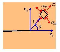Consider an infinite solid, which contains a semi-infinite crack on the (x1,x3) plane. Suppose that the solid deforms in plane strain and is subjected to bounded stress at infinity.  The stress field near the tip of the crack can be derived from the Airy function

$\begin{array}{l}\varphi =\frac{K_I}{3\sqrt{2\pi }}{r}^{3/2}\left(\cos 3\theta /2+3\cos \theta /2\right)\\ -\frac{K_{II}}{\sqrt{2\pi }}{r}^{3/2}\left(\sin 3\theta /2+\sin \theta /2\right)\end{array}$

Here, $K_I$ and $K_{II}$ are two constants, known as mode I and mode II stress intensity factors, respectively.  They quantify the magnitudes of the stresses near the crack tip, as shown below. Their role will be discussed in more detail when we discuss fracture mechanics. The stresses can be calculated as

$\begin{array}{l}{\sigma }_{rr}=\frac{K_I}{\sqrt{2\pi r}}\left(\frac{5}{4}\cos \frac{\theta }{2}-\frac{1}{4}\cos \frac{3\theta }{2}\right)+\frac{K_{II}}{\sqrt{2\pi r}}\left(-\frac{5}{4}\sin \frac{\theta }{2}+\frac{3}{4}\sin \frac{3\theta }{2}\right)\\ {\sigma }_{\theta \theta }=\frac{K_I}{\sqrt{2\pi r}}\left(\frac{3}{4}\cos \frac{\theta }{2}+\frac{1}{4}\cos \frac{3\theta }{2}\right)-\frac{K_{II}}{\sqrt{2\pi r}}\left(\frac{3}{4}\sin \frac{\theta }{2}+\frac{3}{4}\sin \frac{3\theta }{2}\right)\\ {\sigma }_{r\theta }=\frac{K_I}{\sqrt{2\pi r}}\left(\frac{1}{4}\sin \frac{\theta }{2}+\frac{1}{4}\sin \frac{3\theta }{2}\right)+\frac{K_{II}}{\sqrt{2\pi r}}\left(\frac{1}{4}\cos \frac{\theta }{2}+\frac{3}{4}\cos \frac{3\theta }{2}\right)\end{array}$

Equivalent expressions in rectangular coordinates are

$\begin{array}{l}{\sigma }_{11}=\frac{K_I}{\sqrt{2\pi r}}\cos \frac{\theta }{2}\left(1-\sin \frac{\theta }{2}\sin \frac{3\theta }{2}\right)-\frac{K_{II}}{\sqrt{2\pi r}}\sin \frac{\theta }{2}\left(2+\cos \frac{\theta }{2}\cos \frac{3\theta }{2}\right)\\ {\sigma }_{22}=\frac{K_I}{\sqrt{2\pi r}}\cos \frac{\theta }{2}\left(1+\sin \frac{\theta }{2}\sin \frac{3\theta }{2}\right)+\frac{K_{II}}{\sqrt{2\pi r}}\cos \frac{\theta }{2}\sin \frac{\theta }{2}\cos \frac{3\theta }{2}\\ {\sigma }_{12}=\frac{K_I}{\sqrt{2\pi r}}\cos \frac{\theta }{2}\sin \frac{\theta }{2}\cos \frac{3\theta }{2}+\frac{K_{II}}{\sqrt{2\pi r}}\cos \frac{\theta }{2}\left(1-\sin \frac{\theta }{2}\sin \frac{3\theta }{2}\right)\end{array}$

while the displacements can be calculated by integrating the strains, with the result

$\begin{array}{l}{u}_1=\frac{K_I}{\mu }\sqrt{\frac{r}{2\pi }}\left[1-2\nu +{\sin }^2\frac{\theta }{2}\right]\cos \frac{\theta }{2}+\frac{K_{II}}{\mu }\sqrt{\frac{r}{2\pi }}\left[2-2\nu +{\cos }^2\frac{\theta }{2}\right]\sin \frac{\theta }{2}\\ u_2=\frac{K_I}{\mu }\sqrt{\frac{r}{2\pi }}\left[2-2\nu -{\cos }^2\frac{\theta }{2}\right]\sin \frac{\theta }{2}+\frac{K_{II}}{\mu }\sqrt{\frac{r}{2\pi }}\left[-1+2\nu +{\sin }^2\frac{\theta }{2}\right]\cos \frac{\theta }{2}\end{array}$

Note that this displacement field is valid for plane strain deformation only.

 

Observe that the stress intensity factor has the bizarre units of $N{m}^{-3/2}$.