Chapter 9

 

Energy Methods for Linear Elastic Solids

 

 

You may recall that energy methods can often be used to simplify complex problems.  For example, to find the equilibrium configuration of a discrete system, you would begin by identifying a suitable set of generalize coordinates $q_i$, and then express the potential energy in terms of these: $V(q_i)$.  The equilibrium values of the generalized coordinates could then be determined from the condition that the potential energy is stationary at equilibrium: this gives a set of equations $\partial V/\partial q_i=0$ that could be solved for $q_i$.

 

In this section, we will develop an analogous procedure for solving boundary value problems in linear elasticity.  Our generalized coordinates will be the displacement field $u_i(x)$.  We will find an expression for the potential energy of an elastic solid in terms of $u_i$, and then show that the potential energy is stationary if the solid is in equilibrium.  We will find, further, that the potential energy is not only stationary, but is always a minimum, implying that equilibrium configurations in linear elasticity problems are always stable.  (This is because the approximations made in setting up the equations of linear elasticity preclude any possibility of buckling).  This principle will be referred to as the Principle of Minimum Potential Energy. 

 

The main application of the principle is to generate approximate solutions to linear elastic boundary value problems.  Indeed, the principle will form the basis of the Finite Element Method in linear elasticity.

 

 

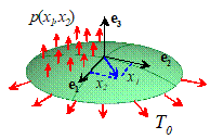
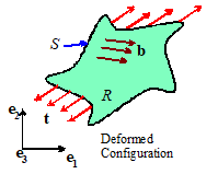In the following, we consider a generic static boundary value problem in linear elasticity, as shown in the picture. 

 

As always, we assume that we are given:

1.      The shape of the solid in its unloaded condition $R$

2.      The initial stress field in the solid (we will take this to be zero)

3.      The elastic constants for the solid $C_{ijkl}$ and its mass density ${\rho }_0$

4.      The thermal expansion coefficients for the solid, and temperature change from the initial configuration $\Delta T$

5.      A body force distribution $b$ (per unit mass) acting on the solid

6.      Boundary conditions, specifying displacements $u^{*}(x)$ on a portion ${\partial }_{1}R$ or tractions on a portion ${\partial }_{2}R$ of the boundary of R

 

 

9.1 Kinematically Admissible Displacement Fields

 

A ‘kinematically admissible displacement field’ $v_i(x)$ is any displacement field with the following properties:

1.      $v_i$ is continuous everywhere within the solid

2.      $v_i$ is differentiable everywhere within the solid, so that a strain field may be computed as

${\widehat{\epsilon }}_{ij}=\frac{1}{2}\left(\frac{\partial v_i}{\partial x_j}+\frac{\partial v_j}{\partial x_i}\right)$

3.      $v_i$ satisfies boundary conditions anywhere that displacements are prescribed, i.e. $v(x)=u^{*}(x)$ on the portion ${\partial }_{1}R$ on the boundary.

 

Note the v is not necessarily the actual displacement in the solid $–$ it is just an arbitrary displacement field which satisfies any displacement boundary conditions.  You can think of it as a possible displacement field that the solid could adopt.  Out of all these possible displacement fields, it will actually select the one that minimizes the potential energy.

 

The kinematically admissible displacement field can also be thought of as a system of generalized coordinates in the context of analytical mechanics.  Recall that, to use a set of generalized coordinates in Lagranges equations, you must make sure that the system of coordinates satisfies all the constraints.  Similarly, to be admissible, our displacement field must satisfy constraints on the boundary. 

 

9.2 Definition of Potential Energy of an Elastic Solid

 

Next, we will define the potential energy of a solid.  The definition may look a bit strange, because it seems to give different values for potential energy depending on how the solid is loaded.  This is true.  But who cares, as long as the definition is useful?

 

For any kinematically admissible displacement field v, the potential energy is

$V(v)={\displaystyle \underset{V}{\int }U(v)}dV-{\displaystyle \underset{V}{\int }{\rho }_0{b}_i{v}_i}dV-{\displaystyle \underset{{\partial }_{2}R}{\int }{t}_i{v}_{i}dA}$

where

$U(v)=\frac{1}{2}{C}_{ijkl}\left({\widehat{\epsilon }}_{ij}-{\alpha }_{ij}\Delta T\right)\left({\widehat{\epsilon }}_{kl}-{\alpha }_{kl}\Delta T\right)$

is the strain energy density associated with the kinematically admissible displacement field. You can interpret the three terms in the formula for V as the strain energy stored inside the solid; the work done by body forces; and the work done by surface tractions. For the particular case of an isotropic material, with $\Delta T=0$, we see that

$U(v)=\frac{E}{2\left(1+\nu \right)}\left({\widehat{\epsilon }}_{ij}{\widehat{\epsilon }}_{ij}+\frac{\nu }{1-2\nu }{\widehat{\epsilon }}_{kk}{\widehat{\epsilon }}_{mm}\right)$

 

 

9.3 The principle of stationary and minimum potential energy.

 

Let v be any kinematically admissible displacement field.  Let u be the actual displacement field $–$ i.e. the one that satisfies the equilibrium equations within the solid as well as all the boundary conditions.  We will show the following:

1. V(v) is stationary (i.e. a local minimum, maximum or inflexion point) for v=u.

2. V(v) is a global minimum for v=u.

 

As a preliminary step, recall that the actual displacement field satisfies the following equations

$\begin{array}{l}{\epsilon }_{ij}=\frac{1}{2}\left(\frac{\partial u_i}{\partial x_j}+\frac{\partial u_j}{\partial x_i}\right){\sigma }_{ij}=C_{ijkl}({\epsilon }_{kl}-{\alpha }_{kl}\Delta T)\frac{\partial {\sigma }_{ij}}{\partial x_i}+{\rho }_0{b}_j=0\\ u_i=u_i^{*}\text{on}{\partial }_{1}R{\sigma }_{ij}{n}_i=t_j^{*}\text{on}{\partial }_{2}R\end{array}$

Next, re-write the kinematically admissible displacement field in terms of u as

$v_i=u_i+\delta u_i$

where $\delta u_i$ is the difference between the kinematically admissible field and the correct equilibrium field.  Observe that

$\begin{array}{l}{v}_i=u_i^{*}{u}_i=u_i^{*}\text{on }{\partial }_{1}R\\ \Rightarrow \delta u_i=0\text{on }{\partial }_{2}R\end{array}$

i.e. the difference between the kinematically admissible field and the actual field is zero wherever displacements are prescribed.

 

Now, note that $V(v)$ can be expressed in terms of $u_i$ and $\delta u_i$ as

$V\left(u+\delta u\right)=V(u)+\delta V+\frac{1}{2}{\delta }^{2}V$

where

$\begin{array}{l}\delta V={\displaystyle \underset{V}{\int }{C}_{ijkl}\left({\epsilon }_{ij}-{\alpha }_{ij}\Delta T\right)\delta {\epsilon }_{kl}dV}-{\displaystyle \underset{V}{\int }{b}_i\delta u_i}dV-{\displaystyle \underset{{\partial }_{2}R}{\int }{t}_i\delta u_{i}dA}{\delta }^{2}V={\displaystyle \underset{V}{\int }{C}_{ijkl}\delta {\epsilon }_{ij}\delta {\epsilon }_{kl}}\\ {\epsilon }_{ij}=\frac{1}{2}\left(\frac{\partial u_i}{\partial x_j}+\frac{\partial u_j}{\partial x_i}\right)\delta {\epsilon }_{ij}=\frac{1}{2}\left(\frac{\partial \delta u_i}{\partial x_j}+\frac{\partial \delta u_j}{\partial x_i}\right)\end{array}$

To see this, simply substitute into the definition of the potential energy

$\begin{array}{l}V(v)={\displaystyle \underset{V}{\int }U(u+\delta u)}dV-{\displaystyle \underset{V}{\int }{b}_i(u_i+\delta u_i)}dV-{\displaystyle \underset{{\partial }_{2}R}{\int }{t}_i(u_i+\delta u_i)dA}\\ ={\displaystyle \underset{V}{\int }\frac{1}{2}{C}_{ijkl}\left({\epsilon }_{ij}-{\alpha }_{ij}\Delta T+\delta {\epsilon }_{ij}\right)\left({\epsilon }_{kl}-{\alpha }_{kl}\Delta T+\delta {\epsilon }_{kl}\right)dV}-{\displaystyle \underset{V}{\int }{b}_i(u_i+\delta u_i)}dV-{\displaystyle \underset{{\partial }_{2}R}{\int }{t}_i(u_i+\delta u_i)dA}\\ \end{array}$

Multiply everything out and use the condition that $C_{ijkl}=C_{klij}$ to get the result stated.

 

Now, to show that $V(v)$ is stationary at v=u, we need to show that $\delta V=0$.  This means that, if we add any small change $\delta u$ to the actual displacement field u, the change in potential energy will be zero, to first order in $\delta u$.

 

To show this, note that

$C_{ijkl}\left({\epsilon }_{ij}-{\alpha }_{ij}\Delta T\right)={\sigma }_{kl}$

Next, note that

${\sigma }_{kl}\delta {\epsilon }_{kl}={\sigma }_{kl}\frac{1}{2}\left(\frac{\partial \delta u_k}{\partial x_l}+\frac{\partial \delta u_l}{\partial x_k}\right)=\frac{1}{2}{\sigma }_{lk}\frac{\partial \delta u_k}{\partial x_l}+\frac{1}{2}{\sigma }_{kl}\frac{\partial \delta u_l}{\partial x_k}={\sigma }_{kl}\frac{\partial \delta u_l}{\partial x_k}$

where we have used the fact that ${\sigma }_{kl}={\sigma }_{lk}$ (angular momentum balance).  Rewrite this as

${\sigma }_{ij}\frac{\partial \delta u_j}{\partial x_i}=\frac{\partial }{\partial x_i}\left({\sigma }_{ij}\delta u_j\right)-\frac{\partial {\sigma }_{ij}}{\partial x_i}\delta u_j$

Substitute back into the expression for  and rearrange to see that

$\delta V={\displaystyle \underset{V}{\int }\frac{\partial }{\partial x_i}\left({\sigma }_{ij}\delta u_j\right)dV}-{\displaystyle \underset{V}{\int }\left(\frac{\partial {\sigma }_{ij}}{\partial x_i}+{\rho }_0{b}_j\right)\delta u_j}dV-{\displaystyle \underset{{\partial }_{2}R}{\int }{t}_i\delta u_{i}dA}$

Now, recall the equations of equilibrium

$\frac{\partial {\sigma }_{ij}}{\partial x_i}+{\rho }_0{b}_j=0$

so that the second term vanishes.  Apply the divergence theorem to express the first integral as a surface integral

${\displaystyle \underset{V}{\int }\frac{\partial }{\partial x_i}\left({\sigma }_{ij}\delta u_j\right)dV={\displaystyle \underset{A}{\int }{\sigma }_{ij}\delta u_j}}{n}_{i}dA$

Recall that $\delta u_i=0\text{on }{\partial }_{1}R$, and note that

${\displaystyle \underset{A}{\int }dA}={\displaystyle \underset{{\partial }_{1}R}{\int }dA}+{\displaystyle \underset{{\partial }_{2}R}{\int }dA}$

because either tractions or displacements (but not both) must be prescribed on every point on the boundary. 

 

Therefore

${\displaystyle \underset{V}{\int }\frac{\partial }{\partial x_i}\left({\sigma }_{ij}\delta u_j\right)dV={\displaystyle \underset{A}{\int }{\sigma }_{ij}\delta u_j}}{n}_{i}dA={\displaystyle \underset{{\partial }_{1}R}{\int }{\sigma }_{ij}{n}_i\delta u_{j}dA}+{\displaystyle \underset{{\partial }_{2}R}{\int }{\sigma }_{ij}{n}_i\delta u_{j}dA}={\displaystyle \underset{{\partial }_{2}R}{\int }{\sigma }_{ij}{n}_i\delta u_{j}dA}$

Finally, recall that

${\sigma }_{ij}{n}_i=t_j\text{on }{\partial }_{2}R$

and substitute back into the expression for $\delta V$ to see that

$\delta V={\displaystyle \underset{{\partial }_{2}R}{\int }\left({\sigma }_{ji}{n}_j-t_i\delta u_i\right)dA}=0$

This proves that V(v) is stationary at v=u, as stated.

 

Finally, we wish to show that V(v) is a minimum at v=u.  This is easy.  Note that we have proved that

$\begin{array}{l}V\left(v\right)=V(u)+\frac{1}{2}{\delta }^{2}V\\ {\delta }^{2}V={\displaystyle \underset{V}{\int }{C}_{ijkl}\delta {\epsilon }_{ij}\delta {\epsilon }_{kl}}\end{array}$

Note that

$\frac{1}{2}{C}_{ijlk}\delta {\epsilon }_{kl}\delta {\epsilon }_{ij}$

is the strain energy density associated with a strain $\delta {\epsilon }_{ij}$.  Strain energy density must always be positive or zero, so that

$V\left(v\right)\ge V(u)$

 

 

 

 

 

 

 

9.4 Useful Formulas for Potential Energy

 

Besides 3D elastic solids, we often use energy methods to analyze solids with special shapes, such as strings, beams, membranes and plates.   These will be discussed in more detail in Section 11, but it is helpful to list formulas for the potential energies of these special solids here, so we can use them in example problems.

 

1-D Axially loaded bar   $\Pi ={{\displaystyle \underset{0}{\overset{L}{\int }}\frac{1}{2}EA\left(\frac{dv}{dx}\right)}}^{2}dx-{\displaystyle \underset{0}{\overset{L}{\int }}q(x)v(x)dx}-Pv(L)$
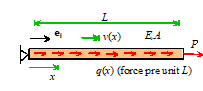
1-D Tensioned Cable $\Pi =T_0{{\displaystyle \underset{0}{\overset{L}{\int }}\frac{1}{2}\left(\frac{dv}{dx}\right)}}^{2}dx-{\displaystyle \underset{0}{\overset{L}{\int }}q(x)v(x)dx}$
1-D Euler-Bernoulli Beam   $\Pi ={{\displaystyle \underset{0}{\overset{L}{\int }}\frac{1}{2}EI\left(\frac{d^{2}v}{d{x}^2}\right)}}^{2}dx-{\displaystyle \underset{0}{\overset{L}{\int }}q(x)v(x)dx}$
2D Biaxially Stretched Membrane   $\Pi ={\displaystyle \underset{A}{\overset{}{\int }}\frac{1}{2}{T}_0}\left[{\left(\frac{\partial v}{\partial x_1}\right)}^2+{\left(\frac{\partial v}{\partial x_2}\right)}^2\right]dA-{\displaystyle \underset{A}{\overset{}{\int }}q(x_1,x_2)v(x_1,x_2)dA}$
2D Kirchhoff Plate   $\begin{array}{l}\Pi =\frac{E{h}^3}{12(1-\nu )}{\displaystyle \underset{A}{\overset{}{\int }}\frac{1}{2}}\left[{\left(\frac{{\partial }^{2}w}{\partial x_1^2}+\frac{{\partial }^{2}w}{\partial x_2^2}\right)}^2-2(1-\nu )\left(\frac{{\partial }^{2}w}{\partial x_1^2}\frac{{\partial }^{2}w}{\partial x_2^2}-{\left(\frac{{\partial }^{2}w}{\partial x_1\partial x_2}\right)}^2\right)\right]dA\\ -{\displaystyle \underset{A}{\overset{}{\int }}q(x_1,x_2)w(x_1,x_2)dA}\end{array}$

 

 

 

 

 

9.5 Uniaxial compression of a cylinder solved by energy methods

 

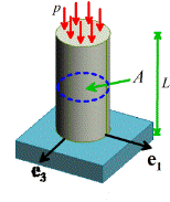Consider a cylindrical bar subjected to a uniform pressure p on one end, and supported on a rigid, frictionless base.  Neglect temperature changes.  Determine the displacement field in the bar.

 

We will solve this problem using energy methods.  We will guess a displacement field of the form

$v_1={\lambda }_1{x}_1,v_2={\lambda }_2{x}_2{v}_3={\lambda }_3{x}_3$

This satisfies the boundary conditions on the bottom face of the cylinder, so it is a kinematically admissible displacement field.  The coefficients ${\lambda }_i$ are to be determined, by minimizing the potential energy.  The strains follow as

${\epsilon }_{11}={\lambda }_1{\epsilon }_{22}={\lambda }_2{\epsilon }_{33}={\lambda }_3$

with all other strain components zero.  The strain energy density is

$U=\frac{E}{2\left(1+\nu \right)}\left\{{\lambda }_1^2+{\lambda }_2^2+{\lambda }_3^2+\frac{\nu }{1-2\nu }{\left({\lambda }_1+{\lambda }_2+{\lambda }_3\right)}^2\right\}$

The boundary conditions are

1.      On the bottom of the cylinder $v_2=0,t_1=t_3=0\Rightarrow v_i{t}_i=0$

2.      On the sides of the cylinder, $t_i=0\Rightarrow v_i{t}_i=0$ 

3.      On the top of the cylinder $v_2(L)={\lambda }_{2}L{t}_2=-p,t_1=t_3=0\Rightarrow v_i{t}_i=-p{\lambda }_{2}L$

Substitute into the expression for strain energy density to see that

$\begin{array}{l}V(v)={\displaystyle \underset{V}{\int }\frac{E}{2\left(1+\nu \right)}\left\{{\lambda }_1^2+{\lambda }_2^2+{\lambda }_3^2+\frac{\nu }{1-2\nu }{\left({\lambda }_1+{\lambda }_2+{\lambda }_3\right)}^2\right\}dV-{\displaystyle \underset{A}{\int }{\lambda }_{2}L(-p)}}\\ =\frac{ALE}{2\left(1+\nu \right)}\left\{{\lambda }_1^2+{\lambda }_2^2+{\lambda }_3^2+\frac{\nu }{1-2\nu }{\left({\lambda }_1+{\lambda }_2+{\lambda }_3\right)}^2\right\}+A{\lambda }_{2}Lp\end{array}$

Now, the actual displacement field minimizes V.  This requires

$\frac{\partial V}{\partial {\lambda }_1}=\frac{\partial V}{\partial {\lambda }_2}=\frac{\partial V}{\partial {\lambda }_3}=0$

Evaluate the derivatives to see that

$\begin{array}{l}\frac{ALE}{2\left(1+\nu \right)}\left\{2{\lambda }_1+\frac{2\nu }{1-2\nu }\left({\lambda }_1+{\lambda }_2+{\lambda }_3\right)\right\}=0\\ \frac{ALE}{2\left(1+\nu \right)}\left\{2{\lambda }_2+\frac{2\nu }{1-2\nu }\left({\lambda }_1+{\lambda }_2+{\lambda }_3\right)\right\}+ALp=0\\ \frac{ALE}{2\left(1+\nu \right)}\left\{2{\lambda }_3+\frac{2\nu }{1-2\nu }\left({\lambda }_1+{\lambda }_2+{\lambda }_3\right)\right\}=0\end{array}$

It is easy to solve these equations to see that

${\lambda }_1=-p/E{\lambda }_2={\lambda }_3=\nu p/E$

 

This is, of course, the exact solution, which is reassuring.  Notice that we never had to calculate stresses or worry about equilibrium $–$ the variational principle takes care of all that for us.

 

Let us solve the same problem, but this time with displacement boundary conditions on the top of the cylinder.

 

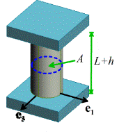The cylinder has unstretched length L and is stretched between frictionless grips to length L+h.  This time, the kinematically admissible displacement field must satisfy boundary conditions on both top and bottom surface of the cylinder.   Therefore, we choose

$v_1={\lambda }_1{x}_1,v_2=h{x}_2/L{v}_3={\lambda }_3{x}_3$

Proceeding as before, we now find that the potential energy is

$V(v)=\frac{ALE}{2\left(1+\nu \right)}\left\{{\lambda }_1^2+\frac{h^2}{L^2}+{\lambda }_3^2+\frac{\nu }{1-2\nu }{\left({\lambda }_1+\frac{h}{L}+{\lambda }_3\right)}^2\right\}$

Note that this time there is no contribution to the potential energy from the tractions on the top of the cylinder, because now the displacement is prescribed there, instead of the pressure.  Minimizing the potential energy as before

$\begin{array}{l}\frac{ALE}{2\left(1+\nu \right)}\left\{2{\lambda }_1+\frac{2\nu }{1-2\nu }\left({\lambda }_1+\frac{h}{L}+{\lambda }_3\right)\right\}=0\\ \frac{ALE}{2\left(1+\nu \right)}\left\{2{\lambda }_3+\frac{2\nu }{1-2\nu }\left({\lambda }_1+\frac{h}{L}+{\lambda }_3\right)\right\}=0\end{array}$

Solve these equations to conclude that

${\lambda }_1={\lambda }_3=-\nu \frac{h}{L}$

Again, this is the exact solution.

 

 

 

 

9.6  Energy methods for calculating stiffness

 

Energy methods can also be used to obtain an upper bound to the stiffness of a structure or a component.

 

Begin by reviewing the meaning of stiffness of an elastic solid.  A spring is an example of an elastic solid.  Recall that if you apply a force P to a spring, it deflects by an amount $\Delta$, in proportion to P.  The stiffness k is defined so that

$k=P/\Delta$

If you apply a load P to any elastic structure (except one which contains two or more contacting surfaces), the point where you apply the load will deflect by a distance that is proportional to the applied load.  For example, for a cantilever beam, the end deflection is

$\Delta =\frac{P{L}^3}{2E{a}^{3}b}$

The stiffness of the beam is therefore $k=P/\Delta =2E{a}^{3}b/L^3$

 

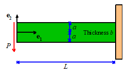
To get an upper bound to the stiffness of a structure, one can merely guess its deformed shape, then apply the principle of minimum potential energy.

 

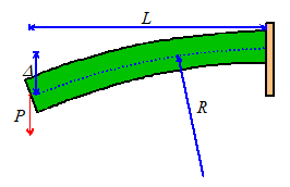
For example, for the beam problem, we might guess that the beam deforms into a circular shape, with unknown radius R.

 

The deflection at the end of the beam is approximately

$\Delta =R-\sqrt{R^2-L^2}\approx \frac{L^2}{2R}$

From the preceding section, we know that the potential energy of a beam is

$V(w)={\displaystyle \underset{0}{\overset{L}{\int }}}\frac{1}{2}EI{\left\{\frac{d^{2}w(x_1)}{d{x}_1{}^2}\right\}}^{2}d{x}_1-{\displaystyle \underset{0}{\overset{L}{\int }}bq(x_1)w(x_1)d{x}_1}$

Here, $q(x_1)=0$, but we need to account for the potential energy of the load P.  Recall that the potential energy of a constant force is $-P\Delta$. Recall also that $d^{2}w/d{x}^2\approx 1/R$. Thus

$V(R)={\displaystyle \underset{0}{\overset{L}{\int }}\frac{1}{2}\frac{EI}{R^2}}d{x}_1-P\Delta =\frac{1}{2}\frac{EI}{R^2}L-P\frac{L^2}{2R}$

Choose R to minimize the potential energy

$\frac{\partial V}{\partial R}=0\Rightarrow -\frac{EI}{R^3}L+P\frac{L^2}{2R^2}=0\Rightarrow R=\frac{2EI}{PL}$

so that

$\Delta =\frac{L^2}{2R}=\frac{L^3}{4EI}P\Rightarrow k\le \frac{4EI}{L^3}$

For comparison, the exact solution is $k=3EI/L^3$

 

 

9.7 Rayleigh-Ritz Method for Calculating Approximate Static Solutions for Elastic Solids

 

The so-called Rayleigh-Ritz method is a formal procedure for obtaining approximate solutions to boundary value problems in elasticity.  It is best illustrated by working through a series of examples, while summarizing the general procedure along the way.

 

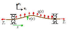
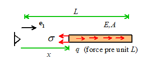
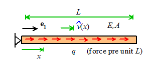Example 1: The bar shown in the figure is loaded by uniform body forces q per unit length.   Estimate the displacement in the bar.

 

1.      Start by guessing an approximate solution that can be progressively improved by adding additional terms.   It is helpful to choose a form for the solution that will (with sufficient terms) interpolate any differentiable function exactly in the limit of an infinite number of terms.   We often use functions such as

$v={\displaystyle \sum _{i=1}^N{a}_i{f}_i(x)}$

where $f_i$  is some a set of basis functions, - examples include

$f_i(x)=x^{i-1}{f}_i(x)=\sin (i-1)\pi x/L$

We can add more and more terms to the polynomial to progressively improve the approximation.  For our present example a polynomial is a good choice, so we choose

$v={\displaystyle \sum _{i=1}^N{a}_i{x}^{i-1}}$

2.      To be a kinematically admissible displacement field, the interpolated approximation must satisfy any boundary conditions.    Here, we require $u(0)=0$, which shows that $a_0=0$ .  More generally, the boundary conditions yield a  set of linear equatinos for the coefficients $a_i$ .   These can be used to eliminate some subset of the unknowns.   It doesn’t matter which ones you eliminate, but it is essential to do the elimination before calculating the potential energy.

3.      Next, we calculate the potential energy.   As an example, let’s choose just one nonzero term $v=a_{2}x$.  The formula for potential energy gives

$\Pi ={{\displaystyle \underset{0}{\overset{L}{\int }}\frac{1}{2}EA\left(\frac{dv}{dx}\right)}}^{2}dx-{\displaystyle \underset{0}{\overset{L}{\int }}q(x)v(x)dx}-Pv(L)=\frac{1}{2}EA{a}_2^{2}L-\frac{1}{2}q{a}_2{L}^2$

4.      Now we minimize the potential energy with respect to all the remaining coefficients in the approximation.  This means the partial derivative with respect to each coefficient in turn must be zero (because the function is stationary).  Here we just have one term

$\frac{\partial \Pi }{\partial a_2}=EAL{a}_2-\frac{q{L}^2}{2}=0$

5.      Solve for all the remaining coefficients

$a_2=\frac{qL}{2EA}\Rightarrow v\approx \frac{qLx}{2EA}$

 

 

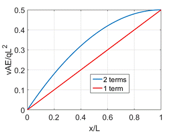
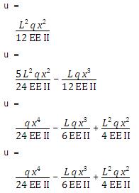
Let’s repeat the procedure but use two terms in the expansion: $v=a_{2}x+a_3{x}^2$.   We can have MATLAB do all the necessary calculus

 

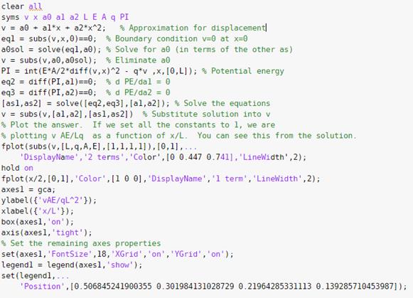
Matlab spits out the solution

The solutions with one and two terms are shown below.

 

To wrap up this discussion, let’s check and see what the exact solution is.   We can easily calculate the stress in the bar: the figure shows a free body diagram for a section created by cutting through the bar at some arbitrary position: this shows that

$A\sigma =q(L-x)$

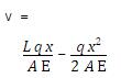
We can then calculate the strain and integrate it to get the displacement

$\epsilon =\frac{\sigma }{E}=\frac{du}{dx}=\frac{q}{AE}(L-x)\Rightarrow u=\frac{qLx}{EA}-\frac{qL{x}^2}{2EA}$

So the Rayleigh-Ritz solution with two terms gives the exact solution.     This is a general result: if the exact solution can be interpolated exactly with a finite number of terms in the approximation, the solution will always yield the exact solution once the appropriate number of terms has been reached.

 

 

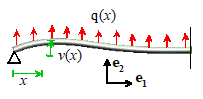
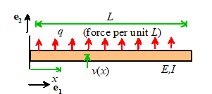Example 2: As a second example we will use the Rayleigh-Ritz method to estimate the solution to a cantilever beam subjected to uniform distributed loading.   We can set up a general MATLAB script to do the calculation automatically for an arbitrary number of terms: the script is shown below.

 

 

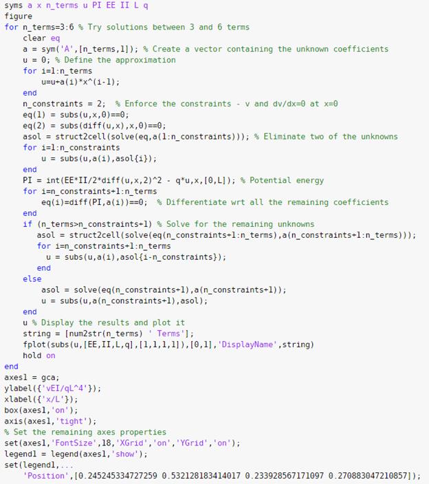
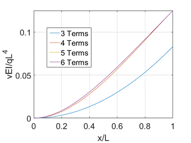
The succession of solutions is shown below $–$ with 5 terms the solution is exact.

 

 

This might give you the impression that we’ve discovered a magic procedure to solve any elasticity problem.   In a sense we have, because the finite element method, which (with a large enough computer) will solve most elasticity problems, is essentially a Rayleigh-Ritz method.   But the analytical approach we’ve used in this section doesn’t always work very well, because symbolic algebra gets very slow with a large number of unknowns.   The finite element method is much more efficient.  This will be the topic of the next section.