Chapter 10

 

Implementing the Finite Element Method for Linear Elasticity

 

 

The goal of this chapter is to provide some insight into the theory and algorithms that are coded in a finite element program.  Here, we will implement only the simplest possible finite element code: specifically, we will develop a finite element method to solve a 2D (plane stress or plane strain) static boundary value problem in linear elasticity, as shown in the picture. 

 

We assume that we are given:

1.      The shape of the solid in its unloaded condition $R$

2.      Boundary conditions, specifying displacements $u^{*}(x)$ on a portion ${\partial }_{1}R$ or tractions on a portion ${\partial }_{2}R$ of the boundary of R

To simplify the problem, we will make the following assumptions

 The solid is an isotropic, linear elastic solid with Young’s modulus E and Poisson’s ratio $\nu$;

 Plane strain or plane stress deformation;

 The solid is at constant temperature (no thermal strains);

 We will neglect body forces.

 

We then wish to find a displacement field $u_i$ satisfying the usual field equations and boundary conditions (see Sect 5.1.1).  The procedure is based on the principle of minimum potential energy discussed in Section 5.7.  There are four steps:

1. A finite element mesh is constructed to interpolate the displacement field
2. The strain energy in each element is calculated in terms of the displacements of each node;
3. The potential energy of tractions acting on the solid’s boundary is added
4. The displacement field is calculated by minimizing the potential energy.

 

These steps are discussed in more detail in the sections below.

 

 

 

10.1 The finite element mesh and element connectivity

 

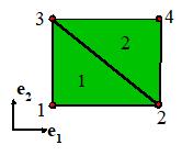
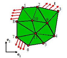
For simplicity, we will assume that the elements are 3 noded triangles, as shown in the picture.  The nodes are numbered 1,2,3…N, while the elements are numbered 1,2…L.  Element numbers are shown in parentheses.

 

The position of the ath node is specified by its coordinates $x_i^{(a)}$

 

The element connectivity specifies the node numbers attached to each element.  For example, in the picture the connectivity for element 1 is (10,9,2); for element 2 it is (10,2,1), etc.

 

 

 

 

 

10.2 The global displacement vector

 

We will approximate the displacement field by interpolating between values at the nodes, as follows.  Let $u_i^{(a)}$ denote the unknown displacement vector at nodes $a=1,2,\mathrm{....}N$.  In a finite element code, the displacements for a plane stress or plane strain problem are normally stored as a column vector like the one shown below:

$\underset{\_}{u}={\left[\begin{array}{cccccccc}{u}_1^{(1)}& u_2^{(1)}& u_1^{(2)}& u_2^{(2)}& u_1^{(3)}& u_2^{(3)}& \dots & \end{array}\right]}^T$

 

The unknown displacement components will be determined by minimizing the potential energy of the solid.

 

 

10.3 Element interpolation functions

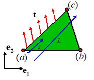
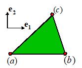
To calculate the potential energy, we need to be able to compute the displacements within each element.  This is done by interpolation.  Consider a triangular element, with nodes a, b, c at its corners. Let $x_i^{(a)},x_i^{(b)},x_i^{(c)}$ denote the coordinates of the corners.  Define the element interpolation functions (also known as shape functions) as follows

$\begin{array}{l}{N}_a(x_1,x_2)=\frac{\left(x_2-x_2^{(b)}\right)\left(x_1^{(c)}-x_1^{(b)}\right)-\left(x_1-x_1^{(b)}\right)\left(x_2^{(c)}-x_2^{(b)}\right)}{\left(x_2^{(a)}-x_2^{(b)}\right)\left(x_1^{(c)}-x_1^{(b)}\right)-\left(x_1^{(a)}-x_1^{(b)}\right)\left(x_2^{(c)}-x_2^{(b)}\right)}\\ N_b(x_1,x_2)=\frac{\left(x_2-x_2^{(c)}\right)\left(x_1^{(a)}-x_1^{(c)}\right)-\left(x_1-x_1^{(c)}\right)\left(x_2^{(a)}-x_2^{(c)}\right)}{\left(x_2^{(b)}-x_2^{(c)}\right)\left(x_1^{(a)}-x_1^{(c)}\right)-\left(x_1^{(b)}-x_1^{(c)}\right)\left(x_2^{(a)}-x_2^{(c)}\right)}\\ N_c(x_1,x_2)=\frac{\left(x_2-x_2^{(a)}\right)\left(x_1^{(b)}-x_1^{(a)}\right)-\left(x_1-x_1^{(a)}\right)\left(x_2^{(b)}-x_2^{(a)}\right)}{\left(x_2^{(c)}-x_2^{(a)}\right)\left(x_1^{(b)}-x_1^{(a)}\right)-\left(x_1^{(c)}-x_1^{(a)}\right)\left(x_2^{(b)}-x_2^{(a)}\right)}\end{array}$

These shape functions are constructed so that

 They vary linearly with position within the element

 Each shape function has a value of one at one of the nodes, and is zero at the other two.

We then write

$u_i(x_1,x_2)=u_i^{(a)}{N}_a(x_1,x_2)+u_i^{(b)}{N}_b(x_1,x_2)+u_i^{(c)}{N}_c(x_1,x_2)$

One can readily verify that this expression gives the correct values for $u_i$ at each corner of the triangle.

 

Of course, the shape functions given are valid only for 3 noded triangular elements $–$ other elements have more complicated interpolation functions.

 

 

10.4 Element strains, stresses and strain energy density

 

We can now compute the strain distribution within the element and hence determine the strain energy density. Since we are solving a plane strain problem, the only nonzero strains are ${\epsilon }_{11},{\epsilon }_{22},{\epsilon }_{12}$.  It is convenient to express the results in matrix form, as follows

$\underset{\_}{\epsilon }=\left[B\right]{\underset{\_}{u}}^{\text{element}}\equiv \left[\begin{array}{c}{\epsilon }_{11}\\ {\epsilon }_{22}\\ 2{\epsilon }_{12}\end{array}\right]=\left[\begin{array}{cccccc}\frac{\partial N_a}{\partial x_1}& 0& \frac{\partial N_b}{\partial x_1}& 0& \frac{\partial N_c}{\partial x_1}& 0\\ 0& \frac{\partial N_a}{\partial x_2}& 0& \frac{\partial N_b}{\partial x_2}& 0& \frac{\partial N_c}{\partial x_2}\\ \frac{\partial N_a}{\partial x_2}& \frac{\partial N_a}{\partial x_1}& \frac{\partial N_b}{\partial x_2}& \frac{\partial N_b}{\partial x_1}& \frac{\partial N_c}{\partial x_2}& \frac{\partial N_c}{\partial x_1}\end{array}\right]\left[\begin{array}{c}{u}_1^{(a)}\\ u_2^{(a)}\\ u_1^{(b)}\\ u_2^{(b)}\\ u_1^{(c)}\\ u_2^{(c)}\end{array}\right]$

The factor of 2 multiplying the shear strains in the strain vector has been introduced for convenience.  Note that, for linear triangular elements, the matrix of shape function derivatives $\left[B\right]$ is constant.  It depends only on the coordinates of the corners of the element, and does not vary with position within the element.  This is not the case for most elements.

 

Now, we can compute the strain energy density within the element.  Begin by computing the stresses within the element.  For plane strain deformation, have that

$\left[\begin{array}{c}{\sigma }_{11}\\ {\sigma }_{22}\\ {\sigma }_{12}\end{array}\right]=\frac{E}{(1+\nu )(1-2\nu )}\left[\begin{array}{ccc}1-\nu & \nu & 0\\ \nu & 1-\nu & 0\\ 0& 0& \frac{1-2\nu }{2}\end{array}\right]\left[\begin{array}{c}{\epsilon }_{11}\\ {\epsilon }_{22}\\ 2{\epsilon }_{12}\end{array}\right]$

For plane stress, the result is

$\left[\begin{array}{c}{\sigma }_{11}\\ {\sigma }_{22}\\ {\sigma }_{12}\end{array}\right]=\frac{E}{(1-{\nu }^2)}\left[\begin{array}{ccc}1& \nu & 0\\ \nu & 1& 0\\ 0& 0& (1-\nu )/2\end{array}\right]\left[\begin{array}{c}{\epsilon }_{11}\\ {\epsilon }_{22}\\ 2{\epsilon }_{12}\end{array}\right]$

Recall (see Sect 3.1.7) that the strain energy density is related to the stresses and strains by $U={\sigma }_{ij}{\epsilon }_{ij}/2$.   This can be written in matrix form as

$U=\frac{1}{2}{\underset{\_}{\epsilon }}^T\underset{\_}{\sigma }=\frac{1}{2}{\underset{\_}{\epsilon }}^T\left[D\right]\underset{\_}{\epsilon }$

where

$\underset{\_}{\sigma }=\left[\begin{array}{c}{\sigma }_{11}\\ {\sigma }_{22}\\ {\sigma }_{12}\end{array}\right]\underset{\_}{\epsilon }=\left[\begin{array}{c}{\epsilon }_{11}\\ {\epsilon }_{22}\\ 2{\epsilon }_{12}\end{array}\right]\left[D\right]=\{\begin{array}{c}\frac{E}{(1+\nu )(1-2\nu )}\left[\begin{array}{ccc}1-\nu & \nu & 0\\ \nu & 1-\nu & 0\\ 0& 0& (1-2\nu )/2\end{array}\right]\text{Plane strain}\\ \frac{E}{(1-{\nu }^2)}\left[\begin{array}{ccc}1& \nu & 0\\ \nu & 1& 0\\ 0& 0& (1-\nu )/2\end{array}\right]\text{Plane stress}\end{array}$

Now, express these results in terms of the nodal displacements for the element

$U^{\text{element}}=\frac{1}{2}{\underset{\_}{u}}^{\text{element}}{}^T\left({\left[B\right]}^T\left[D\right]\left[B\right]\right){\underset{\_}{u}}^{\text{element}}$

We can now compute the total strain energy stored within the element.  Because $\left[B\right]$ is constant, we merely need to multiply the strain energy density by the area of the element, which can be computed from the coordinates of its corners as follows

$A=\frac{1}{2}\left|\left(x_1^b-x_1^a\right)\left(x_2^c-x_2^a\right)-\left(x_1^c-x_1^a\right)\left(x_2^b-x_2^a\right)\right|$

Hence, the total strain energy of the element is

$W^{\text{element}}=\frac{1}{2}{\underset{\_}{u}}^{\text{element}}{}^T\left(A_{\text{element}}{\left[B\right]}^T\left[D\right]\left[B\right]\right){\underset{\_}{u}}^{\text{element}}$

 

10.5 The element stiffness matrix

 

The strain energy can be simplified by defining the element stiffness matrix

$K^{\text{element}}=A_{\text{element}}{\left[B\right]}^T\left[D\right]\left[B\right]$

so that

$W^{\text{element}}=\frac{1}{2}{\underset{\_}{u}}^{\text{element}}{}^T{K}^{\text{element}}{\underset{\_}{u}}^{\text{element}}$

Observe that, because the material property matrix $\left[D\right]$ is symmetric, the element stiffness matrix is also symmetric.  To see this, note that

$K^{\text{element}}{}^T=A_{\text{element}}{\left({\left[B\right]}^T\left[D\right]\left[B\right]\right)}^T=A_{\text{element}}{\left[B\right]}^T{\left[D\right]}^T\left[B\right]=A_{\text{element}}{\left[B\right]}^T\left[D\right]\left[B\right]=K^{\text{element}}$

 

 

10.6 The Global stiffness matrix

 

The total strain energy of the solid may be computed by adding together the  strain energy of each element:

$W={\displaystyle \sum _{\text{elements}}{W}^{\text{element}}}=\frac{1}{2}{\displaystyle \sum _{\text{elements}}{\underset{\_}{u}}^{\text{element}}{}^T{K}^{\text{element}}{\underset{\_}{u}}^{\text{element}}}$

It is more convenient to express W in terms of the vector  which contains all the nodal displacements, rather than using ${\underset{\_}{u}}^{\text{element}}$ for each element to describe the displacements.  For example, the strain energy for the simple 2 element mesh shown is

$\begin{array}{l}W=\frac{1}{2}\left[\begin{array}{cccccc}{u}_1^{(1)}& u_2^{(1)}& u_1^{(2)}& u_2^{(2)}& u_1^{(3)}& u_2^{(3)}\end{array}\right]\left[\begin{array}{cccc}{k}_{11}^{(1)}& k_{12}^{(1)}& \cdots & k_{16}^{(1)}\\ k_{21}^{(1)}& k_{22}^{(1)}& & \\ ⋮& & \ddots & \\ k_{61}^{(1)}& & & k_{66}^{(1)}\end{array}\right]\left[\begin{array}{c}{u}_1^{(1)}\\ u_2^{(1)}\\ u_1^{(2)}\\ u_2^{(2)}\\ u_1^{(3)}\\ u_2^{(3)}\end{array}\right]\\ +\frac{1}{2}\left[\begin{array}{cccccc}{u}_1^{(2)}& u_2^{(2)}& u_1^{(3)}& u_2^{(3)}& u_1^{(4)}& u_2^{(4)}\end{array}\right]\left[\begin{array}{cccc}{k}_{11}^{(2)}& k_{12}^{(2)}& \cdots & k_{16}^{(2)}\\ k_{21}^{(2)}& k_{22}^{(2)}& & \\ ⋮& & \ddots & \\ k_{61}^{(2)}& & & k_{66}^{(2)}\end{array}\right]\left[\begin{array}{c}{u}_1^{(2)}\\ u_2^{(2)}\\ u_1^{(3)}\\ u_2^{(3)}\\ u_1^{(4)}\\ u_2^{(4)}\end{array}\right]\end{array}$

If we wanted to, we could add the missing terms to each element displacement vector:

$\begin{array}{l}W=\frac{1}{2}\\ \left[\begin{array}{cccccc}{u}_1^{(1)}& u_2^{(1)}& u_1^{(2)}& u_2^{(2)}& u_1^{(3)}& u_2^{(3)}\end{array}\begin{array}{cc}{u}_1^{(4)}& u_2^{(4)}\end{array}\right]\\ \left[\begin{array}{cccccccc}{k}_{11}^{(1)}& k_{12}^{(1)}& k_{13}^{(1)}& k_{14}^{(1)}& & \cdots & 0& 0\\ k_{21}^{(1)}& k_{22}^{(1)}& k_{32}^{(1)}& & & & 0& 0\\ & & k_{33}^{(1)}& k_{34}^{(1)}& & & 0& 0\\ & & k_{43}^{(1)}& k_{44}^{(1)}& & & 0& 0\\ & & k_{53}^{(1)}& & & & 0& 0\\ & & ⋮& & & \ddots & 0& 0\\ 0& 0& 0& 0& 0& 0& 0& 0\\ 0& 0& 0& 0& 0& 0& 0& 0\end{array}\right]\left[\begin{array}{c}\begin{array}{l}{u}_1^{(1)}\\ u_2^{(1)}\\ u_1^{(2)}\end{array}\\ u_2^{(2)}\\ u_1^{(3)}\\ u_2^{(3)}\\ u_1^{(4)}\\ u_2^{(4)}\end{array}\right]\\ +\left[\begin{array}{cccccc}{u}_1^{(1)}& u_2^{(1)}& u_1^{(2)}& u_2^{(2)}& u_1^{(3)}& u_2^{(3)}\end{array}\begin{array}{cc}{u}_1^{(4)}& u_2^{(4)}\end{array}\right]\\ \left[\begin{array}{cccccccc}0& 0& 0& 0& 0& \cdots & 0& 0\\ 0& 0& 0& 0& 0& & 0& 0\\ 0& 0& k_{11}^{(2)}& k_{12}^{(2)}& & & & \\ 0& 0& k_{21}^{(2)}& k_{22}^{(2)}& & & & \\ 0& 0& k_{31}^{(2)}& & & & & \\ 0& 0& & & & \ddots & & \\ 0& 0& ⋮& & & & & k_{56}^{(2)}\\ 0& 0& & & & & k_{65}^{(2)}& k_{66}^{(2)}\end{array}\right]\left[\begin{array}{c}\begin{array}{l}{u}_1^{(1)}\\ u_2^{(1)}\\ u_1^{(2)}\end{array}\\ u_2^{(2)}\\ u_1^{(3)}\\ u_2^{(3)}\\ u_1^{(4)}\\ u_2^{(4)}\end{array}\right]\end{array}$

We can now collect together corresponding terms in the two element stiffness matrices to express this as

$\begin{array}{l}W=\frac{1}{2}\left[\begin{array}{cccccc}{u}_1^{(1)}& u_2^{(1)}& u_1^{(2)}& u_2^{(2)}& u_1^{(3)}& u_2^{(3)}\end{array}\begin{array}{cc}{u}_1^{(4)}& u_2^{(4)}\end{array}\right]\\ \left[\begin{array}{cccccccc}{k}_{11}^{(1)}& k_{12}^{(1)}& k_{13}^{(1)}& k_{14}^{(1)}& & \cdots & & \\ k_{21}^{(1)}& k_{22}^{(1)}& k_{32}^{(1)}& & & & & \\ & & k_{33}^{(1)}+k_{11}^{(2)}& k_{34}^{(1)}+k_{12}^{(2)}& & & & \\ & & k_{43}^{(1)}+k_{21}^{(2)}& k_{44}^{(1)}+k_{22}^{(2)}& & & & \\ & & k_{53}^{(1)}+k_{31}^{(2)}& & & & & \\ & & & & & \ddots & & \\ & & ⋮& & & & & k_{56}^{(2)}\\ & & & & & & k_{65}^{(2)}& k_{66}^{(2)}\end{array}\right]\left[\begin{array}{c}\begin{array}{l}{u}_1^{(1)}\\ u_2^{(1)}\\ u_1^{(2)}\end{array}\\ u_2^{(2)}\\ u_1^{(3)}\\ u_2^{(3)}\\ u_1^{(4)}\\ u_2^{(4)}\end{array}\right]\end{array}$

 We can therefore write

$W=\frac{1}{2}{\underset{\_}{u}}^T\left[K\right]\underset{\_}{u}$

where $\left[K\right]$ is known as the Global stiffness matrix.  It is the sum of all the element stiffness matrices.

 

Because the element stiffness matrix is symmetric, the global stiffness matrix must also be symmetric.

 

To assemble the global stiffness matrix for a plane strain or plane stress mesh with N nodes, we use the following procedure.

 

1.      Note that for $N$ nodes, there will be $2N$ unknown displacement components (2 at each node).  Therefore, we start by setting up storage for a $\left(2N\times 2N\right)$ global stiffness matrix, and set each term in the matrix to zero.

2.      Next, begin a loop over the elements.

3.      For the current element, assemble the element stiffness matrix

$K^{\text{element}}=A_{\text{element}}{\left[B\right]}^T\left[D\right]\left[B\right]$

4.      Add the element stiffness matrix to the global stiffness matrix, using the following procedure.  Let a, b, c denote the numbers of the nodes on the 3 corners of the element.  Let $k_{ij}^{\text{element}}$ for i=1…6, j=1…6  denote the terms in the the element stiffness matrix.  Let $K_{nm}$ for n=1…2N, m=1…2N denote the terms in the global stiffness matrix.  Then,

$\begin{array}{l}{K}_{2a-1,2a-1}+=k_{11}^{\text{element}},K_{2a-1,2a}+=k_{12}^{\text{element}}\\ K_{2a-1,2b-1}+=k_{13}^{\text{element}}{K}_{2a-1,2b}+=k_{14}^{\text{element}}\\ K_{2a-1,2c-1}+=k_{15}^{\text{element}}{K}_{2a-1,2c}+=k_{16}^{\text{element}}\\ \\ K_{2a,2a-1}+=k_{21}^{\text{element}},K_{2a,2a}+=k_{22}^{\text{element}}\\ K_{2a,2b-1}+=k_{23}^{\text{element}}{K}_{2a,2b}+=k_{24}^{\text{element}}\\ K_{2a,2c-1}+=k_{25}^{\text{element}}{K}_{2a,2c}+=k_{26}^{\text{element}}\\ \\ K_{2b-1,2a-1}+=k_{31}^{\text{element}},K_{2b-1,2a}+=k_{32}^{\text{element}}\\ K_{2b-1,2b-1}+=k_{33}^{\text{element}}{K}_{2b-1,2b}+=k_{34}^{\text{element}}\\ K_{2b-1,2c-1}+=k_{35}^{\text{element}}{K}_{2b-1,2c}+=k_{36}^{\text{element}}\\ ⋮\\ K_{2c,2a-1}+=k_{61}^{\text{element}},K_{2c,2a}+=k_{62}^{\text{element}}\\ K_{2c,2b-1}+=k_{63}^{\text{element}}{K}_{2c,2b}+=k_{64}^{\text{element}}\\ K_{2c,2c-1}+=k_{65}^{\text{element}}{K}_{2c,2c}+=k_{66}^{\text{element}}\end{array}$

Here, the symbol += means that the term on the left is incremented by the term on the right, following standard C syntax.

 

5. Proceed to the next element.

10.7 Boundary loading

 

We have now found a way to compute the strain energy for a finite  element mesh.  Next, we need to compute the boundary term in the potential energy.

 

Boundary loading will be specified as follows:

1. The element on which the loading acts

2. The face of the element which is loaded

3. The traction vector t (force per unit area) that acts on the face of the element.  The traction is assumed to be constant on the face of any one element.

 

Now, we compute the contribution to the potential energy due to the traction acting on the face of one element.

 

For the element shown, the contribution to the potential energy would be

$P=-{\displaystyle \underset{0}{\overset{L}{\int }}{t}_i{u}_{i}ds}$

Recall that the displacements vary linearly within a 3 noded triangle.  Therefore, we can write

$u_i=u_i^{(a)}\frac{s}{L}+u_i^{(c)}\left(1-\frac{s}{L}\right)$

So, since the tractions are uniform

$\begin{array}{l}{P}^{\text{element}}=-t_i{u}_i^{(a)}{\displaystyle \underset{0}{\overset{L}{\int }}\frac{s}{L}ds}-t_i{u}_i^{(c)}{\displaystyle \underset{0}{\overset{L}{\int }}\left(1-\frac{s}{L}\right)ds}\\ =-t_i{u}_i^{(a)}\frac{L}{2}-t_i{u}_i^{(c)}\frac{L}{2}\\ =-\left[\begin{array}{cccc}{t}_1\frac{L}{2}& t_2\frac{L}{2}& t_1\frac{L}{2}& t_2\frac{L}{2}\end{array}\right]\cdot \left[\begin{array}{cccc}{u}_1^{(a)}& u_2^{(a)}& u_1^{(c)}& u_2^{(c)}\end{array}\right]\end{array}$

Abbreviate this as

$P^{\text{element}}=-{\underset{\_}{r}}^{\text{face}}\cdot {\underset{\_}{u}}^{\text{face}}$

 

 

10.8 Global force vector

 

The total contribution to the potential energy due to boundary loading on all element faces is

$P=-{\displaystyle \sum _{\text{faces}}{\underset{\_}{r}}^{\text{faces}}\cdot {\underset{\_}{u}}^{\text{faces}}}$

It is more convenient to express this in terms of the global displacement vector $\underset{\_}{u}$

$P=-\underset{\_}{r}\cdot \underset{\_}{u}$

where  is the global residual force vector.

 

The global residual force vector for a mesh with N nodes is assembled as follows.

1.      The residual force vector has length 2N (2 entries per node).  Reserve storage for a vector of length 2N and initialize to zero

2.      Loop over elements

3.      Determine which face of the element is loaded.  Let a, b denote the node numbers attached to this face.  Determine the residual force vector for the element face.  Let $r_i{}^{\text{face}}$, i=1…4 denote the terms in the element face residual vector.  Let $r_n$, n=1…2N denote the terms in the global residual force vector.  Then

$\begin{array}{l}{r}_{2a-1}+=r_1^{\text{face}}{r}_{2a}+=r_2^{\text{face}}\\ r_{2b-1}+=r_3^{\text{face}}{r}_{2b}+=r_4^{\text{face}}\end{array}$

 

 

 

10.9 Minimizing the Potential Energy

 

We have set up the following expression for the potential energy of a finite element mesh

$\begin{array}{l}V=\frac{1}{2}{\underset{\_}{u}}^T\left[K\right]\underset{\_}{u}-\underset{\_}{r}\cdot \underset{\_}{u}\\ \equiv \frac{1}{2}{\displaystyle \sum _{j=1}^{2N}{u}_j{\displaystyle \sum _{i=1}^{2N}{K}_{ji}{u}_i}}-{\displaystyle \sum _{j=1}^{2N}{r}_j{u}_j}\end{array}$

Now, minimize V

$\frac{\partial V}{\partial u_k}=\frac{1}{2}{\displaystyle \sum _{i=1}^{2N}{K}_{ki}{u}_i}+\frac{1}{2}{\displaystyle \sum _{j=1}^{2N}{u}_j{K}_{jk}}-r_k=0$

where we have noted that

$\frac{\partial u_j}{\partial u_k}=\{\begin{array}{l}1,j=k\\ 0,j\ne k\end{array}$

Simplify this by noting that $\left[K\right]$ is symmetric

$\begin{array}{l}\frac{\partial V}{\partial u_k}=\frac{1}{2}{\displaystyle \sum _{i=1}^{2N}{K}_{ki}{u}_i}+\frac{1}{2}{\displaystyle \sum _{j=1}^{2N}{u}_j{K}_{kj}}-r_k\\ ={\displaystyle \sum _{i=1}^{2N}{K}_{ki}{u}_i}-r_k=0\\ \Rightarrow \left[K\right]\underset{\_}{u}=\underset{\_}{r}\end{array}$

This is a system of 2N simultaneous linear equations for the 2N unknown nodal displacements.  Standard computational techniques such as Gaussian elimination, Cholesky factorization or conjugate gradient methods may be used to solve the system of equations.

 

 

 

 

 

 

 

 

10.10 Eliminating prescribed displacements

 

So far, we have seen how to calculate displacements in a finite element mesh which is subjected to prescribed loading.  What if displacements are prescribed instead?

 

If this is the case, the stiffness matrix and residual are first assembled exactly as described in the preceding section.  They are then modified to enforce the constraint.  The procedure is best illustrated using an example. Suppose that the finite element equations after assembly have the form

$\left[\begin{array}{cccc}{k}_{11}& k_{12}& \cdots & k_{12N}\\ k_{21}& k_{22}& & k_{22N}\\ ⋮& & \ddots & \\ k_{2N1}& k_{2N2}& & k_{2N2N}\end{array}\right]\left[\begin{array}{c}{u}_1^{(1)}\\ u_2^{(1)}\\ ⋮\\ u_2^{(N)}\end{array}\right]=\left[\begin{array}{c}{r}_1\\ r_2\\ ⋮\\ r_4\end{array}\right]$

To prescribe displacements for any node, we simply replace the equation for the appropriate degrees of freedom with the constraint.  For example, to force $u_2^{(1)}=\Delta$, we could modify the finite element equations to

$\left[\begin{array}{cccc}{k}_{11}& k_{12}& \cdots & k_{12N}\\ 0& 1& & 0\\ ⋮& & \ddots & \\ k_{2N1}& k_{2N2}& & k_{2N2N}\end{array}\right]\left[\begin{array}{c}{u}_1^{(1)}\\ u_2^{(1)}\\ ⋮\\ u_2^{(N)}\end{array}\right]=\left[\begin{array}{c}{r}_1\\ \Delta \\ ⋮\\ r_4\end{array}\right]$

Thus, the equation for $u_2^{(1)}$ has been replaced with the constraint $u_2^{(1)}=\Delta$.

 

This procedure works, but has the disadvantage that the modified stiffness matrix is no longer symmetric.  It is preferable to modify the stiffness and residual further, to retain symmetry.  To do so, we eliminate the constrained degrees of freedom from all rows of the stiffness matrix. This is best illustrated by example.  Suppose our modified stiffness matrix has the form

$\left[\begin{array}{cccc}{k}_{11}& k_{12}& \cdots & k_{12N}\\ 0& 1& & 0\\ ⋮& & \ddots & \\ k_{2N1}& k_{2N2}& & k_{2N2N}\end{array}\right]\left[\begin{array}{c}{u}_1^{(1)}\\ u_2^{(1)}\\ ⋮\\ u_2^{(N)}\end{array}\right]=\left[\begin{array}{c}{r}_1\\ \Delta \\ ⋮\\ r_4\end{array}\right]$

Now, we wish to set each entry in the second column (apart from the diagonal) to zero, so that the stiffness is symmetric.  Recall that we can add and subtract equations in the system from one another without affecting the solution.  Therefore, to symmetrize the stiffness matrix in our example, we can subtract appropriate multiples of the second row so as to set each entry in the second column to zero.

$\left[\begin{array}{cccc}{k}_{11}& 0& \cdots & k_{12N}\\ 0& 1& & 0\\ ⋮& & \ddots & \\ k_{2N1}& 0& & k_{2N2N}\end{array}\right]\left[\begin{array}{c}{u}_1^{(1)}\\ u_2^{(1)}\\ ⋮\\ u_2^{(N)}\end{array}\right]=\left[\begin{array}{c}{r}_1-k_{12}\Delta \\ \Delta \\ ⋮\\ r_4-k_{2N2}\Delta \end{array}\right]$

 

 

 

10.11 Solution

 

The result of Sections 10.1-10.10 is a set of simultaneous linear equations of the form

$\left[K^{\mathrm{mod}}\right]\underset{\_}{u}=\underset{\_}{r}$

These can be solved for the unknown displacements $\underset{\_}{u}$ using standard techniques (e.g. Gaussian elimination or iterative techniques).  An important feature of the FEM equations is that the stiffness matrix is sparse $–$ that is to say, only a small number of entries in the matrix are non-zero.  Consequently, special schemes are used to store and factor the equations, which avoid having to store large numbers of zeros. 

 

10.12 Post-processing

 

Once the displacements have been computed, the strain in each element can be computed, and so the stress distribution can be deduced.  The procedure is as follows

1.      For the element of interest, extract the displacement of each node from the global displacement vector

2.      Calculate the strains using the procedure in 7.2.4

$\underset{\_}{\epsilon }=\left[B\right]{\underset{\_}{u}}^{\text{element}}\equiv \left[\begin{array}{c}{\epsilon }_{11}\\ {\epsilon }_{22}\\ 2{\epsilon }_{12}\end{array}\right]=\left[\begin{array}{cccccc}\frac{\partial N_a}{\partial x_1}& 0& \frac{\partial N_b}{\partial x_1}& 0& \frac{\partial N_c}{\partial x_1}& 0\\ 0& \frac{\partial N_a}{\partial x_2}& 0& \frac{\partial N_b}{\partial x_2}& 0& \frac{\partial N_c}{\partial x_2}\\ \frac{\partial N_a}{\partial x_2}& \frac{\partial N_a}{\partial x_1}& \frac{\partial N_b}{\partial x_2}& \frac{\partial N_b}{\partial x_1}& \frac{\partial N_c}{\partial x_2}& \frac{\partial N_c}{\partial x_1}\end{array}\right]\left[\begin{array}{c}{u}_1^{(a)}\\ u_2^{(a)}\\ u_1^{(b)}\\ u_2^{(b)}\\ u_1^{(c)}\\ u_2^{(c)}\end{array}\right]$

3.      The stresses can then be determined from the stress-strain equations

$\underset{\_}{\sigma }=\left[D\right]\underset{\_}{\epsilon }$

where $[D]$ is defined in 7.2.4.

 

10.13 Example FEA code

 

A simple MATLAB implementation of the procedure is provided in the file FEM_conststrain_m.

 

The code reads an input file.  A very simple input file (with just two elements) can be found in FEM_conststrain_input.txt. A second data file

 

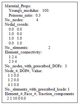
The data file solves the problem illustrated in the picture.  A rectangular block with Young’s modulus 100 and Poisson’s ratio 0.3 is meshed with two elements.  Node 1 is pinned; node 4 is constrained against horizontal motion, and the right hand face of element 2 is subjected to a constant horizontal traction with magnitude 10. 

The input file is shown below $–$ it should be mostly self-explanatory. 

 

Note that

1.      Nodes are numbered sequentially $–$ thus node (1) has coordinates (0,0); node (2) has coordinates (1,0), etc.

2.      The element connectivity specifies the node numbers attached to each element, using a counterclockwise numbering convention.  It doesn’t matter which node you use for the first one, as long as all the others are ordered in a counterclockwise sense around the element. For example, you could use (2,4,1) instead of (1,2,4) for the connectivity of the first element.

3.      To fix motion of a node, you need to enter the node number, the degree of freedom that is being constrained,  (1 for horizontal, 2 for vertical), and a value for the prescribed displacement.

4.      To specify tractions acting on an element face, you need to enter (a) the element number; (b) the face number of the element, and (c,d) the horizontal and vertical components of traction acting on the face.  The face numbering scheme is determined by the element connectivity, as follows.  Face (1) has the first and second nodes as end points; face (2) has the second and third nodes; and face (3) has the third and first nodes as end points.  Since connectivity for element (2) was entered as (2,3,4), face 1 of this element has nodes numbered 2 and 3; face 2 connects nodes numbered 3 and 4, while face 3 connects nodes numbered 4 and 1.

 and enter a name for the output file.

1.      Return to the top of the file, and press <enter> to execute each MAPLE block. If all goes well, you should see that, after reading the input data, MAPLE plots the mesh (just as a check). 

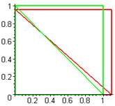
2.      If you continue to the end, you should see a plot of the displaced mesh (red) superimposed on the original mesh (green), as shown on the right.

3.      Finally, open the output file.  It should contain the results shown below