Chapter 2
Introduction to Finite Element Analysis
in Solid Mechanics
Most practical design calculations involve components
with a complicated three-dimensional geometry, and may also need to account for
inherently nonlinear phenomena such as contact, large shape changes, or
nonlinear material behavior. These
problems can only be solved using computer simulations. The finite element method is by far the most widely
used and versatile technique for simulating deformable solids. This chapter gives a brief overview of the
finite element method, with a view to providing the background needed to run
simple simulations using a commercial finite element program. More advanced analysis requires a deeper
understanding of the theory and implementation of finite element codes, which
will be addressed in the next chapter.
HEALTH
WARNING: It is deceptively easy to
use commercial finite element software: most programs come with a nice
user-interface that allows you to define the geometry of the solid, choose a material
model, generate a finite element mesh and apply loads to the solid with a few
mouse clicks. If all goes well, the
program will magically turn out animations showing the deformation; contours
showing stress distributions; and much more besides. It is all too easy, however, to produce
meaningless results, by attempting to solve a problem that does not have a well
defined solution; by using an inappropriate numerical scheme; or simply using
incorrect settings for internal tolerances in the code. In addition, even high quality software can
contain bugs. Always treat the results
of a finite element computations with skepticism!
2.1 Introduction
The finite element method (FEM) is a computer
technique for solving partial differential equations. One application is to predict the deformation
and stress fields within solid bodies subjected to external forces. However, FEM can also be used to solve
problems involving fluid flow, heat transfer, electromagnetic fields,
diffusion, and many other phenomena.
 The principle objective of the displacement based
finite element method is to compute the displacement
field within a solid subjected to external forces.
The principle objective of the displacement based
finite element method is to compute the displacement
field within a solid subjected to external forces.
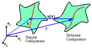
To make this precise, visualize a solid deforming
under external loads. Every point in the
solid moves as the load is applied. The
displacement vector u(x) specifies the motion of the point at position x in the undeformed solid.
Our objective is to determine u(x). Once u(x)
is known, the strain and stress fields in the solid can be deduced.
There are two general types of finite element analysis
in solid mechancis. In most cases, we
are interested in determining the behavior of a solid body that is in static equilibrium. This means that both external and internal
forces acting on the solid sum to zero.
In some cases, we may be interested in the dynamic behavior of a solid body.
Examples include modeling vibrations in structures, problems involving
wave propagation, explosive loading and crash analysis.
For Dynamic
Problems the finite element method solves the equations of motion for a
continuum essentially a more complicated version of . Naturally, in this case it must calculate the motion of the solid as a
function of time.
For Static
Problems the finite element method solves the equilibrium equations . In this case, it may not be necessary to
calculate the time variation of motion.
However, some materials are history dependent (e.g metals deformed in
the plastic regime). In addition, a
static equilibrium problem may have more than one solution, depending on the
load history. In this case the time
variation of the solution must be computed.
For some applications, you may also need to solve
additional field equations. For example,
you may be interested in calculating the temperature distribution in the solid,
or calculating electric or magnetic fields.
In addition, special finite element procedures are available to
calculate buckling loads and their modes, as well as natural frequencies of
vibration and the corresponding mode shapes for a deformable solid.
To
set up a finite element calculation, you
will need to specify
1. The geometry of the solid. This is done by generating a finite element mesh for the solid. The mesh can usually be generated
automatically from a CAD representation of the solid.
2. The properties of the material. This is done by specifying a constitutive law for the solid.
3. The nature of the loading applied to the solid. This is done by specifying the boundary conditions for the problem.
4. If your
analysis involves contact between two more more solids, you will need to
specify the surfaces that are likely to come into contact, and the properties
(e.g. friction coefficient) of the contact.
5. For a dynamic analysis, it is necessary to specify initial conditions for the
problem. This is not necessary for a
static analysis.
6. For problems involving additional fields, you may need
to specify initial values for these field variables (e.g. you would need to
specify the initial temperature distribution in a thermal analysis).
You will also need to specify some additional aspects
of the problem you are solving and the solution procedure to be used:
1. You will need to specify whether the computation should take into
account finite changes in the geometry of the solid.
2. For a dynamic analysis, you will need to specify the time period
of the analysis (or the number of time increments)
3. For a static analysis you will need to decide whether the problem is
linear, or nonlinear. Linear problems
are very easy to solve. Nonlinear
problems may need special procedures.
4. For a static analysis
with history dependent materials you will need to specify the time period of
the analysis, and the time step size (or number of steps)
5. If you are
interested in calculating natural frequencies and mode shapes for the system,
you must specify how many modes to extract.
6. Finally, you will need to specify what the
finite element method must compute.
The
steps in running a finite element computation are discussed in more detail in
the following sections.
2.2 The
Finite Element Mesh for a 2D or 3D component
The finite element mesh is used to specify the
geometry of the solid, and is also used to describe the displacement field
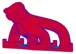
within the solid. A typical mesh (generated
in the commercial FEA code ABAQUS) is shown in the picture to the right.
A finite element mesh may be three dimensional, like
the example shown. Two dimensional
finite element meshes are also used to model simpler modes of deformation. There are three main types of two dimensional
finite element mesh:
1. Plane stress
2. Plane strain
3. Axisymmetric
 In addition, special types of finite element can be
used to model the overall behavior of a 3D solid, without needing to solve for
the full 3D fields inside the solid.
Examples are shell elements; plate elements; beam elements and truss
elements. These will be discussed in a
separate section below.
In addition, special types of finite element can be
used to model the overall behavior of a 3D solid, without needing to solve for
the full 3D fields inside the solid.
Examples are shell elements; plate elements; beam elements and truss
elements. These will be discussed in a
separate section below.
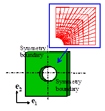
 Plane
Stress Finite Element Mesh : A plane stress finite element mesh is used to
model a plate - like solid which is loaded in its own plane. The solid must have uniform thickness, and
the thickness must be much less than any representative cross sectional
dimension. A plane stress finite element
mesh for a thin plate containing a hole is shown in the figure to the right. Only on quadrant of the specimen is modeled,
since symmetry boundary conditions will be enforced during the analysis.
Plane
Stress Finite Element Mesh : A plane stress finite element mesh is used to
model a plate - like solid which is loaded in its own plane. The solid must have uniform thickness, and
the thickness must be much less than any representative cross sectional
dimension. A plane stress finite element
mesh for a thin plate containing a hole is shown in the figure to the right. Only on quadrant of the specimen is modeled,
since symmetry boundary conditions will be enforced during the analysis.

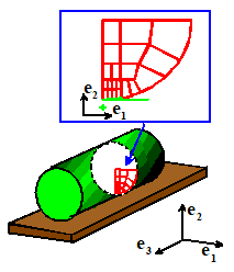 Plane Strain finite element mesh : A
plane strain finite element mesh is used to model a long cylindrical solid that
is prevented from stretching parallel to its axis. For example, a plane strain finite element
mesh for a cylinder which is in contact with a rigid floor is shown in the
figure. Away from the ends of the
cylinder, we expect it to deform so that the out of plane component of
displacement . There is no need to solve for ,
therefore, so a two dimensional mesh is sufficient to calculate and .
Plane Strain finite element mesh : A
plane strain finite element mesh is used to model a long cylindrical solid that
is prevented from stretching parallel to its axis. For example, a plane strain finite element
mesh for a cylinder which is in contact with a rigid floor is shown in the
figure. Away from the ends of the
cylinder, we expect it to deform so that the out of plane component of
displacement . There is no need to solve for ,
therefore, so a two dimensional mesh is sufficient to calculate and .
As before, only one quadrant of the specimen is
meshed: symmetry boundary conditions will be enforced during the analysis.
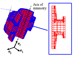 Axisymmetric finite element mesh: An
axisymmetric mesh is used to model a solids that has rotational symmetry, which
is subjected to axisymmetric loading. An
example is shown on the right.
Axisymmetric finite element mesh: An
axisymmetric mesh is used to model a solids that has rotational symmetry, which
is subjected to axisymmetric loading. An
example is shown on the right.
The picture compares a three dimensional mesh of an
axisymmetric bushing to an axisymmetric mesh.
Note that the half the bushing has been cut away in the 3D view, to show
the geometry more clearly. In an
axisymmetric analysis, the origin for the (x,y)
coordinate system is always on the axis of
rotational symmetry. Note also
that to run an axisymmetric finite element analysis, both the geometry of the
solid, and also the loading applied to the solid, must have rotational symmetry
about the y axis.
2.2.1 Nodes and Elements in a Mesh
 A finite element mesh is defined by a set of nodes together with a set of finite elements, as shown in the sketch on
the right.
A finite element mesh is defined by a set of nodes together with a set of finite elements, as shown in the sketch on
the right.
Nodes: The
nodes are a set of discrete points within the solid body. Nodes have the following properties:
1. A node
number. Every node is assigned an integer number,
which is used to identify the node. Any
convenient numbering scheme may be selected the nodes do not need to be numbered in order,
and numbers may be omitted. For example,
one could number a set of n nodes as
100, 200, 300… 100n, instead of
1,2,3…n.
2. Nodal
coordinates. For a three dimensional finite element
analysis, each node is assigned a set of
coordinates, which specifies the position of
the node in the undeformed solid. For a
two dimensional analysis, each node is assigned a pair of coordinates.
For an axisymmetric analysis, the axis must coincide with the axis of rotational
symmetry.
3. Nodal
displacements. When the solid deforms, each node moves to a
new position. For a three dimensional
finite element analysis, the nodal displacements specify the three components
of the displacement field u(x) at each node: . For a two dimensional analysis, each node has
two displacement components . The nodal displacements are unknown at the
start of the analysis, and are computed by the finite element program.
4. Other nodal
degrees of freedom. For more complex
analyses, we may wish to calculate a temperature distribution in the solid, or
a voltage distribution, for example. In
this case, each node is also assigned a temperature, voltage, or similar quantity
of interest. There are also some finite
element procedures which use more than just displacements to describe shape
changes in a solid. For example, when
analyzing two dimensional beams, we use the displacements and rotations of the
beam at each nodal point to describe the deformation. In this case, each node has a rotation, as
well as two displacement components. The
collection of all unknown quantities (including displacements) at each node are
known as degrees of freedom. A finite element program will compute values
for these unknown degrees of freedom.
Elements
are used to partition the solid into discrete regions. Elements have the following properties.
1. An element
number. Every element is assigned an integer number,
which is used to identify the element.
Just as when numbering nodes, any convenient scheme may be selected to
number elements.
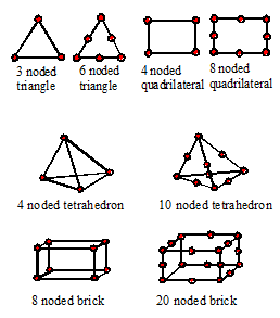
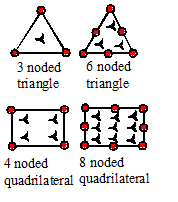
2. A geometry. There are many
possible shapes for an element. A few of
the more common element types are shown in the picture. Nodes attached to the element are shown in
red. In two dimensions, elements are
generally either triangular or rectangular. In three dimensions, the elements
are generally tetrahedra, hexahedra or bricks.
There are other types of element that are used for special purposes:
examples include truss elements (which are simply axial members), beam
elements, and shell elements.
3. A set of
faces. These are simply the sides of the element.
4. A set of
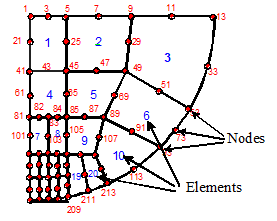
nodes attached to the element. The picture on the right shows a typical
finite element mesh. Element numbers are
shown in blue, while node numbers are shown in red (some element and node
numbers have been omitted for clarity).
All the elements are 8 noded quadrilaterals. Note that each element is connected to a set
of nodes: element 1 has nodes (41, 45, 5, 1, 43, 25, 3, 21), element 2 has
nodes (45, 49, 9, 5, 47, 29, 7, 25), and so on.
It is conventional to list the nodes the nodes in the order given, with
corner nodes first in order going counterclockwise around the element, followed
by the midside nodes. The set of nodes
attached to the element is known as the element
connectivity.
5. An element
interpolation scheme. The purpose of a finite element is to
interpolate the displacement field u(x)
between values defined at the nodes.
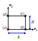
This is best illustrated using an example. Consider the two dimensional, rectangular 4
noded element shown in the figure. Let ,
,
,
denote the components of displacement at nodes
a, b, c, d. The displacement at an arbitrary point within
the element can be interpolated between values at the corners, as follows
where
You can verify for yourself that the displacements
have the correct values at the corners of the element, and the displacements
evidently vary linearly with position within the element.
Different types of element interpolation scheme
exist. The simple example described
above is known as a linear
element. Six noded triangles and 8 noded
triangles are examples of quadratic
elements: the displacement field varies quadratically with position within the
element. In three dimensions, the 4
noded tetrahedron and the 8 noded brick are linear elements, while the 10 noded
tet and 20 noded brick are quadratic.
Other special elements, such as beam elements or shell elements, use a
more complex procedure to interpolate the displacement field.
Some special types of element interpolate both the
displacement field and some or all components of the stress field within an
element separately. (Usually, the displacement interpolation is sufficient to
determine the stress, since one can compute the strains at any point in the
element from the displacement, and then use the stressstrain relation
for the material to find the stress). This type of element is known as a hybrid element. Hybrid elements are usually used to model
incompressible, or nearly incompressible, materials.
6. Integration
points. One objective of a finite element analysis is
to determine the distribution of stress within a solid. This is done as follows. First, the displacements at each node are
computed (the technique used to do this will be discussed in Section 7.2 and
Chapter 8.) Then, the element
interpolation functions are used to determine the displacement at arbitrary
points within each element. The
displacement field can be differentiated to determine the strains. Once the strains are known, the stressstrain relations
for the element are used to compute the stresses.
In principle, this procedure could be used to
determine the stress at any point within an element. However, it turns out to work better at some
points than others. The special points
within an element where stresses are computed most accurately are known as integration points. (Stresses are sampled at these points in the
finite element program to evaluate certain volume and area integrals, hence
they are known as integration points).
For a detailed description of the locations of
integration points within an element, you should consult an appropriate user
manual. The approximate locations of
integration points for a few two dimensional elements are shown in the figure.
There are some special types of element that use fewer
integration points than those shown in the picture. These are known as reduced integration elements. This type of element is usually less
accurate, but must be used to analyze deformation of incompressible materials
(e.g. rubbers or rigid plastic metals).
7. A stressstrain relation
and material properties. Each element is occupied by solid
material. The type of material within
each element (steel, concrete, soil, rubber, etc) must be specified, together
with values for the appropriate material properties (mass density, Young’s
modulus, Poisson’s ratio, etc).
 2.2.2 Special
Elements Beams, Plates, Shells and Truss elements
2.2.2 Special
Elements Beams, Plates, Shells and Truss elements
If you need to analyze a solid with a special geometry
(e.g. a simple truss, a structure made of one or more slender beams, or plates)
it is not efficient to try to generate a full 3D finite element mesh for each
member in the structure. Instead, you
can take advantage of the geometry to simplify the analysis.
The idea is quite simple. Instead of trying to calculate the full 3D
displacement field in each member, the deformation is characterized by a
reduced set of degrees of freedom.
Specifically:
1. For a pin jointed truss, we simply calculate the displacement of each joint in the
structure. The members are assumed to be in a state of uniaxial tension or
compression, so the full displacement field within each member can be
calculated in terms of joint displacements.
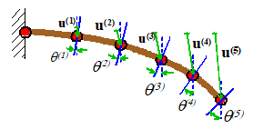
2. For a beam, we calculate the displacement and rotation of the cross section along the beam. These can be used to determine the internal
shear forces bending moments, and therefore the stresses in the beam. A three
dimensional beam has 3 displacement and 3 rotational degrees of freedom at each
node.
3.  For a plate, or shell, we again calculate the displacement and rotation of the plate
section. A three dimensional plate or shell has 3 displacement and two rotational degrees of freedom at
each node (these rotations characterize the rotation of a unit vector normal to
the plate). In some finite element
codes, nodes on plates and shells have a fictitious third rotational degree of
freedom which is added for convenience but you will find that attempting to impose
boundary conditions on this fictitious degree of freedom has no effect on the
deformation of the structure.
For a plate, or shell, we again calculate the displacement and rotation of the plate
section. A three dimensional plate or shell has 3 displacement and two rotational degrees of freedom at
each node (these rotations characterize the rotation of a unit vector normal to
the plate). In some finite element
codes, nodes on plates and shells have a fictitious third rotational degree of
freedom which is added for convenience but you will find that attempting to impose
boundary conditions on this fictitious degree of freedom has no effect on the
deformation of the structure.
In
an analysis using truss, beam or plate elements, some additional information
must be specified to set up the problem:
1. For a truss analysis, each member in the truss is a
single element. The area of the member’s
cross section must be specified.
2. For a beam analysis, the shape and orientation of the
cross section must be specified (or, for an elastic analysis, you could specify
the area moments of inertia directly).
There are also several versions of beam theory, which account
differently for shape changes within the beam.
Euler-Bernoulli beam theory is the simple version covered in
introductory courses. Timoshenko beam
theory is a more complex version, which is better for thicker beams.
3. For plates and shells, the thickness of the plate must
be given. In addition, the deformation
of the plate can be approximated in various ways for example, some versions only account for
transverse deflections, and neglect in-plane shearing and stretching of the
plate; more complex theories account for this behavior.
Calculations using beam and plate theory also differ
from full 3D or 2D calculations in that both the deflection and rotation of the beam or plate must
be calculated. This means that:
1. Nodes on beam elements have 6 degrees of freedom the three displacement components, together
with three angles representing rotation of the cross-section about three axes. Nodes on plate or shell elements have 5 (or
in some FEA codes 6) degrees of freedom.
The 6 degrees of freedom represent 3 displacement components, and two
angles that characterize rotation of the normal to the plate about two axes (if
the nodes have 6 degrees of freedom a third, fictitious rotation component has
been introduced you will have to read the manual for the code
to see what this rotation represents).
2. Boundary conditions may constrain both displacement
and rotational degrees of freedom. For
example, to model a fully clamped boundary condition at the end of a beam (or
the edge of a plate), you must set all displacements and all rotations to zero.
3.
You can apply
both forces and moments to nodes in an analysis.
Finally,
in an analysis involving several beams connected together, you can connect the
beams in two ways:
1. You can connect them with a pin joint, which forces the beams to move together at the
connection, but allows relative rotation
2. You can connect them with a clamped joint, which forces the beams to rotate together at the
connection.
In most FEA codes, you can create the joints by adding
constraints, as discussed in Section 1.2.6 below. Occasionally, you may also
wish to connect beam elements to solid, continuum elements in a model: this can
also be done with constraints.
2.3 Material
Behavior
 A good finite element code contains a huge library of
different types of material behavior that may be assigned to elements. A few examples are described below.
A good finite element code contains a huge library of
different types of material behavior that may be assigned to elements. A few examples are described below.
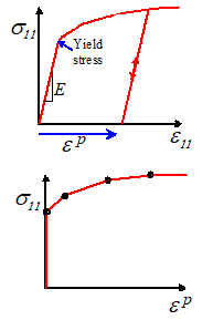
Linear
Elasticity. You should alreadly be
familiar with the idea of a linear elastic material. It has a uniaxial stressstrain response
(valid only for small strains) as shown in the picture
The
stress--strain law for the material may be expressed in matrix form as
Here, E and v are Young’s modulus and Poisson’s
ratio for the material, while denotes the thermal expansion coefficient. Typical values (for steel) are E=210 GN/ , v=0.33, .
 Elasticplastic material
behavior is usually used to model metals that are subjected to large
stresses, but there are also versions of plastic stress-strain laws that model
soils and concrete.
Elasticplastic material
behavior is usually used to model metals that are subjected to large
stresses, but there are also versions of plastic stress-strain laws that model
soils and concrete.
An elastic-plastic material behaves elastically until
a critical stress (known as the yield stress) is reached. If yield is exceeded, the material deforms
permanently. The yield stress of the matierial
generally increases with plastic strain: this behavior is known as strain hardening.
The conditions necessary to initiate yielding under
multiaxial loading are specified by a yield
criterion, such as the Von-Mises or Tresca criteria. These yield criteria are built into the
finite element code.
The strain hardening behavior of a material is
approximated by allowing the yield stress to increase with plastic strain. The variation of yield stress with plastic
strain for a material is usually specified by representing it as a series of
straight lines, as shown in the picture.
A typical yield stress for a metal might vary from
80Mpa (for a material like pure aluminum) to 1 GPa (for a high-strength steel).
Hyperelasticity
is intended to model rubbery materials (or elastomeric foams, like a sponge)
which have (i) a reversible stress-v-strain relation and (ii) the stress is
independent of strain rate or loading history.
They are intended to model large changes in shape of the material
(that’s what the ‘hyper’ refers to).
This means that the stress-v-strain relation has to be defined rather
carefully, because there are several choices of stress and strain measure (e.g.
we could use ‘true’ stress or ‘nominal’ stress; similarly we could use
‘engineering’ strain or ‘true’ strain).
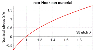 The simplest hyperelastic material model is the
so-called ‘neo-Hookean’ material. This model
is intended to predict the behavior of rubbers, which resist volume changes,
but deform very easily when subjected to shear stress. It has two material properties: (i) a shear
modulus , and (ii) a bulk modulus K. The bulk modulus is
always much greater than the shear modulus and (especially in hand
calculations) is often assumed to be infinite (which means the material is
incompressible). In uniaxial tension,
an incompressible neo-Hookean material has a uniaxial stress-v-stretch relation
of the form
The simplest hyperelastic material model is the
so-called ‘neo-Hookean’ material. This model
is intended to predict the behavior of rubbers, which resist volume changes,
but deform very easily when subjected to shear stress. It has two material properties: (i) a shear
modulus , and (ii) a bulk modulus K. The bulk modulus is
always much greater than the shear modulus and (especially in hand
calculations) is often assumed to be infinite (which means the material is
incompressible). In uniaxial tension,
an incompressible neo-Hookean material has a uniaxial stress-v-stretch relation
of the form
where is the nominal stress (force per unit undeformed
area) in the specimen, and is the ratio of deformed length to original
length of the specimen. The curve is
shown in the figure.
A typical value for the shear modulus of a rubber
might be 0.5MPa.
Linear
Viscoelasticity is used to model polymers or biological tissues that are
subjected to modest strains (less than 0.5%).
A typical application might be to model the energy dissipation during
cyclic loading of a polymeric vibration damper, or to model human tissue
responding to an electric shaver.
Viscoelastic
materials have a time-dependent response, which can be measured in two
different ways:
1. Take a specimen that is free of stress at time ,
apply a constant shear stress for and measuring the resulting shear strain as a function of time. The results are generally presented by
plotting the `creep compliance’ as a function of time.
2.
Take a specimen that is
free of stress at time ,
apply a constant shear strain for and measuring the resulting shear stress as a function of time. In this case the
results are presented by plotting the Relaxation Modulus:
Similar
experiments can be done to measure the response of the material to pressure (or
volume changes) but in many practical applications the time-dependence of the
pressure or volume is negligible, and the material can be assumed to have a
constant bulk modulus.
In
finite element simulations the time dependence of shear (and if necessary bulk)
modulus is usually specified by entering values for the so-called ‘Prony
series’ for the material
where is the steady-state stiffness (represented by the
parallel spring), and are a set of time constants and stiffnesses. The Prony series can be interpreted as a
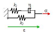
complicated spring-damper model for the material behavior. For example, the spring-damper system shown
in the figure is a useful simple viscoelastic mode. It has a Prony series
2.4 Boundary
conditions, Constraints, Interfaces and Contact
Boundary conditions are used to specify the loading
applied to a solid. There are several
ways to apply loads to a finite element mesh:
Displacement
boundary conditions. The
displacements at any node on the boundary or within the solid can be
specified. One may prescribe ,
,
,
or all three. For a two dimensional
analysis, it is only necessary to prescribe and/or .
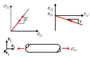
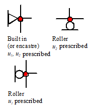
Various symbols are used to denote displacement
boundary conditions applied to a finite element mesh: a few of these are illustrated
in the figure on the right. Some
user-interfaces use small conical arrowheads to indicate constrained displacement
components.
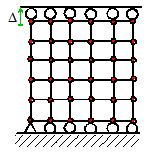
For example, to stretch a 2D block of material
vertically, while allowing it to expand or contract freely horizontally, we
would apply boundary constraints to the top and bottom surface as shown in the
figure.
Observe that one of the nodes on the bottom of the
block has been prevented from moving horizontally, as well as vertically. It is important to do this: the finite
element program will be unable to find a unique solution for the displacement
fields if the solid is free to slide horizontally.
During the analysis, the finite element program will
apply forces to the nodes with prescribed displacements, so as to cause them to
move to their required positions. If
only the component of displacement is prescribed, then
the force will act in the direction.
If is prescribed, the force acts in direction ,
and so on. Notice that you cannot directly apply a rotation to a node attached to a 2D or 3D solid. Rotations can, however, be applied to the
nodes attached to certain special types of element, such as beams, plates and
shells, as well as rigid surfaces.
Symmetry
conditions: Most finite element codes can automatically enforce symmetry
and anti-symmetry boundary conditions.
Prescribed
forces. Any node in a finite element mesh may be subjected to a prescribed
force. The nodal force is a vector, and
is specified by its three (or two for 2D) components, . Notice there is no direct way to apply a moment to a 3D solid you would need to do this by applying two
point forces a small distance apart, or by applying contact loading, as
outlined below. Moments can be applied
to some special types of element, such as shells, plates or beams.
Distributed
loads. A solid may be subjected to
distributed pressure or traction acting on ints boundary. Examples include aerodynamic loading, or
hydrostatic fluid pressure. Distributed traction is a vector quantity, with physical dimensions of
force per unit area in 3D, and force per unit length in 2D. To model this type of loading in a finite
element program, distributed loads may be applied to the the face of any
element.
Default
boundary condition at boundary nodes.
If no displacements or forces are prescribed at a boundary node, and no
distributed loads act on any element faces connected to that node, then the
node is assumed to be free of external force.
Body
forces. External body forces may act
on the interior of a solid. Examples of
body forces include gravitational loading, or electromagnetic forces. Body force is a vector quantity, with
physical dimensions of force per unit volume.
To model this type of loading in a finite element program, body forces
may be applied to the interior of any element.
Contact. Probably the most common way to load a solid
is through contact with another solid.
Special procedures are available for modeling contact between solids these will be discussed in a separate section
below.
 Load
history. In some cases, one may wish
to apply a cycle of load to a solid. In
this case, the prescribed loads and displacements must be specified as a
function of time.
Load
history. In some cases, one may wish
to apply a cycle of load to a solid. In
this case, the prescribed loads and displacements must be specified as a
function of time.
General
guidelines concerning boundary conditions.
When performing a static analysis, it is very important to make sure
that boundary conditions are applied properly.
A finite element program can only solve a problem if a unique static
equilibrium solution to the problem exists.
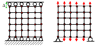
Difficulties arise if the user does not specify sufficient
boundary constraints to prevent rigid body motion of a solid. This is best illustrated by example. Suppose we wish to model stretching a 2D
solid, as described earlier. The
examples to the right show two correct ways to do this.
The examples below show various incorrect ways to
apply boundary conditions. In each case,
one or more rigid body mode is unconstrained.
2.4.1 Constraints
You may sometimes need to use more complicated
boundary conditions than simply constraining the motion or loads applied to a
solid. Some examples might be
1.
Connecting
different element types, e.g. beam elements to solid elements;
2.
Enforcing
periodic boundary conditions
3.
Constraining a
boundary to remain flat
4.
Approximating the
behavior of mechanical components such as welds, bushings, bolted joints, etc.
You can do this by defining constraints in an analysis.
At the most basic level, constraints can simply be used to enforce
prescribed relationships between the displacements or velocities of individual
nodes in the mesh. You can also specify
relationships between motion of groups
of nodes.
2.4.2 Contacting Surfaces and Interfaces
In addition to being subject to forces or prescribed
displacements, solid objects are often loaded by coming into contact with
another solid.
Modern finite element codes contain sophisticated
capabilities for modeling contact.
Unfortunately, contact can make a computation much more difficult,
because the region where the two solids come into contact is generally not
known a priori, and must be
determined as part of the solution. This
almost always makes the problem nonlinear
even if both contacting solids are linear
elastic materials. In addition, if there
is friction between the contacting solids, the solution is history dependent.
For
this reason, many options are available in finite element packages to control
the way contacting surfaces behave.
There
are three general cases of contact that you may need to deal with:
1. A deformable solid contacts a stiff, hard solid whose
deformation may be neglected. In this
case the hard solid is modeled as a rigid
surface, as outlined below.
2.
You may need to
model contact between two deformable solids
3. The solid comes into contact with itself during the
course of deformation (this is common in components made from rubber, for
example, and also occurs during some metal forming operations).
Whenever
you model contact, you will need to
1. Specify pairs of surfaces that might come into
contact. One of these must be designated
as the master surface and the other
must be designated as the slave surface. (If
a surface contacts itself, it is both a master and a slave. Kinky!)
2. Define the way the two surfaces interact, e.g. by
specifying the coefficient of friction between them.
Modeling
a stiff solid as a rigid surface: In
many cases of practical interest one of the two contacting solids is much more
compliant than the other. Examples
include a rubber in contact with metal, or a metal with low yield stress in
contact with a hard material like a ceramic.
As long as the stresses in the stiff or hard solid are not important,
its deformation can be neglected.
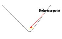
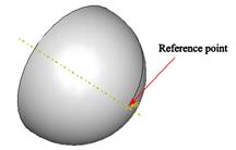
In
this case the stiffer of the two solids may be idealized as a rigid surface. Both 2D and 3D rigid surfaces can be created,
as shown in the figure.
A rigid surface (obviously) can’t change its shape,
but it can move about and rotate. Its
motion is defined using a reference point
on the solid, which behaves like a node.
To move the solid around during an analyisis, you can define
displacement and rotational degrees of freedom at this node. Alternatively, you could apply forces and
moments to the reference point.
Finally, in a dynamic analysis, you can give the rigid solid appropriate
inertial properties (so as to create a rigid projectile, for example).
 Defining
a contact pair master/slave surfaces: Whenever you set up
a finite element calculation that involves contact, you need to specify pairs
of surfaces that may come into contact during the analysis. One of each pair must be designated the master surface, the other must be
designated the slave surface.
Defining
a contact pair master/slave surfaces: Whenever you set up
a finite element calculation that involves contact, you need to specify pairs
of surfaces that may come into contact during the analysis. One of each pair must be designated the master surface, the other must be
designated the slave surface.
This rather obscure finite element terminology refers
to the way that contact constraints are actually applied during a
computation. The geometry of the master
surface will be interpolated as a smooth curve in some way (usually by
interpolating between nodes). The slave
surface is not interpolated. Instead,
each individual node on the slave surface is constrained so as not to penetrate
into the master surface. For example,
the red nodes on the slave surface shown in the figure would be forced to
remain outside the red boundary of the master surface.
For a sufficiently fine mesh, the results should not
be affected by your choice of master and slave surface. However, it improves convergence (see below to learn what this means) if you choose the
more rigid of the two surfaces to be the master surface. If you don’t know which surface is more
rigid, just make a random choice. If you
run into convergence problems later, try switching them over.
Contact
parameters You can define several parameters that control the behavior of
two contacting surfaces:
1. The contact formulation - `finite sliding’ or `small
sliding’ specifies the expected relative tangential
displacement of the two surfaces.
`Finite sliding’ is the most general, but is computationally more
demanding. `Small sliding’ should be
used if the relative tangential displacement is likely to be less than the
distance between two adjacent nodes.
2. You can specify the relationship between the contact
pressure and separation between the contacting surfaces. Alternatively, you can
assume the contact is `hard’ this means the interface can’t withstand any
tension, and the two contacting surfaces cannot inter-penetrate.
3.
You can specify
the tangential behavior of the interface for example by giving the friction
coefficient.
2.5 Initial
Conditions and external fields
For a dynamic analysis, it is necessary to specify the
initial velocity and displacement of each node in the solid. The default value is zero velocity and
displacement.
In addition, if you are solving a coupled problem one involving coupled deformation and heat
flow, for example - you may need to specify initial values for the additional
field variables (e.g. the temperature distribution)
2.6 Solution
procedures and time increments
The finite element method calculates the displacement at each node in the finite element mesh by
solving the equations of static equilibrium or the equations of motion. In this section, we briefly outline some of
the solution procedures, and the options available to control them.
Linear
or Nonlinear Geometry As you know, you can simplify the calculation of
internal forces in a structures by neglecting shape changes when solving the
equations of equilibrium. For example,
when you solve a truss problem, you usually calculate forces in each member
based on the undeformed shape of the
structure.
You can use the same idea to simplify calculations
involving deformable solids. In general,
you should do so whenever possible.
However, if either
1. You anticipate that material might stretch by more
than 10% or so or
2. You expect that some part of the solid might rotate by
more than about 10 degrees
3. You wish to calculate buckling loads for your
structure
you should account for finite geometry changes in the
computation. This will automatically
make your calculation nonlinear (and so more difficult), even if all the
materials have linear stress-strain relations.
Time
stepping for dynamic problems: For a dynamic problem, the nodal
displacements must be calculated as a function of
time. The displacements are calculated
by solving the equations of motion for the system, which look something like
where M and
K are called mass and stiffness
matrices. Both M and K can be functions
of u. There are 2.5 ways to integrate this
equation.
1. The most direct method is called explicit time integration, or explicit
dynamics and works something like this.
Remember that for a dynamic calculation, the values of u and are known at t=0. We can therefore
compute M and K at time t=0, and then
use them to calculate the acceleration at t=0,
as
The acceleration can
then be used to find the velocity and displacement at time as
This procedure can
then be applied repeatedly to march the solution through time.
2. The second procedure is called implicit time integration or implicit
dynamics. The procedure is very
similar to explicit time integration, except that instead of calculating the
mass and stiffness matrices at time t=0,
and using them to calculate acceleration at t=0,
these quantities are calculated at time instead.
This is a bit more time consuming to do, however, because it involves
more equation solving.
3. The 2.5th method is called Modal Dynamics and only works if M and K are constant. In this
case one can take the Fourier transform of the governing equation and integrate
it exactly. This method is used to solve
linear vibration problems.
The
following guidelines will help you to choose the most appropriate method for
your application:
1. For explicit
dynamics each time step can be calculated very fast. However, the method is stable only if is very small specifically, the time interval must be
smaller than the time taken for an elastic wave to propagate from one side of
an element to the other. This gives ,
where is the mass density of the solid, is its shear modulus and its Poisson’s ratio. Explicit dynamics works best for rapid,
transient problems like crash dynamics or impact. It is not good for modeling processes that
take place over a long time. If elastic
wave propagation is not the main focus of your computation, you can sometime
speed up the calculations by increasing the density (but you have to be careful to make sure this
does not affect the results). This is
called mass scaling.
2. For implicit
dynamics the cost of computing each time step is much greater. The algorithm is unconditionally stable,
however, and will always converge even for very large . This is the method of choice for problems
where inertial loading is important, but rapid transients are not the focus of
the analysis.
3. Modal
Dynamics only works for linear
elastic problems. It is used for
vibration analysis.
Nonlinear
Solution Procedures for Static Problems: If a problem involves contact,
plastically deforming materials, or large geometry changes it is nonlinear. This means that the equations of static
equilibrium for the finite element mesh have the general form
where F() denotes
a set of b=1,2…N vector functions of
the nodal displacements ,
a=1,2…N, and N is the number of nodes in the mesh.
The nonlinear equations are solved using the
Newton-Raphson method, which works like this.
You first guess the solution to the equations say . Of course (unless you are a genius) w won’t satisfy the equations, so you
try to improve the solution by adding a small correction . Ideally, the correction should be chosen so
that
but
of course it’s not possible to do this.
So instead, take a Taylor
expansion to get
The result is a system of linear equations of the form
,
where is a constant matrix called the stiffness matrix. The equations can now be solved for ;
the guess for w can be corrected,
and the procedure applied over again.
The iteration is repeated until ,
where is a small tolerance.
In problems involving hard contact, an additional iterative method is used to decide
which nodes on the slave surface contact the master surface. This is just a brute-force method it starts with some guess for contacting
nodes; gets a solution, and checks it.
If any nodes are found to penetrate the master surface, these are added
to the list of nodes in contact. If any
nodes are experiencing forces attracting them to the master surface, they are
removed from the list of nodes in contact.
The problem with any iterative procedure is that it
may not converge that is, repeated corrections either take the solution further and further
away from the solution, or else just spiral around the solution without every
reaching it.
The solution is (naturally) more likely to converge if
the guess is close to the correct solution. Consequently, it is best to apply the loads
to a nonlinear solid gradually, so that at each load step the displacements are
small. The solution to one load
increment can then be used as the initial guess for the next.
Convergence problems are the curse of FEM
analysts. They are very common and can
be exceedingly difficult to resolve.
Here are some suggestions for things to try if you run into convergence
problems:
1. Try applying the load in smaller increments. most commercial codes will do this this
automatically but will stop the computation if the increment
size falls below a minimum value. You
can try reducing the minimum step size..
2. Convergence problems are sometimes caused by ill conditioning in the stiffness
matrix. This means that the equations cannot be solved accurately. Ill conditioning can arise because of (i)
severely distorted elements in the mesh; (ii) material behavior is
incompressible, or nearly incompressible; and (iii) The boundary conditions in
the analysis do not properly constrain the solid. You can fix (i) by modifying
the mesh some FEM codes contain capabilities to
automatically remove element distorsion during large deformation. You can avoid
problems with incompressibility (ii) by using reduced integration elements or
hybrid elements. Problems with boundary
conditions (iii) can usually be corrected by adding more constraints. There is one common problem where this is
hard to do if the motion of a body in your analysis is
constrained only by contacts with other solids (e.g. a roller between two surfaces)
the stiffness matrix is always singular at the start of the analysis. Some finite element codes contain special
procedures to deal with this problem.
3. Try to isolate the source of the problem. Convergence issues can often be traced to one
or more of the following: (i) Severe material nonlinearity; (ii) Contact and
(iii) Geometric nonlinearity. Try to
change your model to remove as many of these as possible e.g. if you are doing a plasticity computation
with contact and geometric nonlinearity, try doing an elastic calculation and
see if it works. If so, the problems are
caused by material nonlinearity.
Similarly, try analyzing the two contacting solids separately, without
the contact; or try the computation without nonlinear geometry. Once you’ve traced the source of the problem,
you might be able to fix it by changing the material properties, contact
properties or loading conditions.
4. Convergence problems are often caused by some kind of
mechanical or material failure in the solid, which involve a sudden release of
energy. In this case, the shape of the
solid may suddenly jump from one static equilibrium configuration to another,
quite different, equilibrium configuration.
There is a special type of loading procedure (called the Riks method) that
can be used to stabilize this kind of problem.
5. Some boundary value problems have badly behaved
governing equations. For example, the
equations governing plane strain deformation of a perfectly plastic solid
become hyperbolic for sufficiently large strains. Static FEM simply won’t work for these
problems. Your best bet is to try an
explicit dynamic calculation instead, perhaps using mass scaling to speed up
the calculation.
 Load steps and increments: When you set
up a finite element model, you usually apply the load in a series of
steps. You can define different boundary
conditions in each step. Unless you
specify otherwise, the loads (or displacements) will vary linearly from their
values at the start of the step to their values at the end of the step, as
illustrated in the picture.
Load steps and increments: When you set
up a finite element model, you usually apply the load in a series of
steps. You can define different boundary
conditions in each step. Unless you
specify otherwise, the loads (or displacements) will vary linearly from their
values at the start of the step to their values at the end of the step, as
illustrated in the picture.
In a nonlinear analysis, the solution may not converge
if the load is applied in a single increment.
If this is the case, the load must be applied gradually, in a series of
smaller increments. Many finite element
codes will automatically reduce the time step if the solution fails to
converge.
2.7 Output
The finite element method always calculates the displacement of each node in the mesh these are the unknown variables in the
computation. However, these may not be
the quantities you are really interested in.
A number of quantities can be computed from the displacement fields,
including:
1. Velocity and acceleration fields
2. Strain components, principal strains, and strain
invariants,or their rates
3. Elastic and plastic strains or strain rates
4. Stress components; principal stresses; stress
invariants
5. Forces applied to nodes or boundaries
6. Contact pressures
7. Values of material state variables (e.g. yield
stresses)
8. Material failure criteria
All these quantities can be computed as functions of
time at selected points in the mesh (either at nodes, or at element integration
points); as functions of position along paths connecting nodes; or as contour
plots.
2.8 Units in finite element computations, using dimensional analysis
A finite element code merely solves the equations of
motion (or equilibrium), together with any equations governing material
behavior. Naturally, equations like F=ma
and do not contain any units a priori. Consequently, when
entering geometric dimensions, material data and loads into an FEA code, you can use any system of units you like,
but the units of all quantities must be consistent. You have to be very careful with this. When you sketch the part you are modeling, it
is often convenient to enter dimensions in cm, inches, or mm. This is fine but then cm,
inches or mm must be used for any other material or load data that contain
length dimensions. For example, if
you use cm to dimension your part, then you must enter data for Young’s modulus
and yield stress in ,
and you must also specify pressures acting on the system in . In this case, the FEA code will report
stresses in units of .
Using
Dimensional Analysis to simplify FEA analysis.
 You may have used dimensional analysis to find
relationships between data measured in an experiment (especially in fluid
mechanics). The same idea can be used to
relate variables you might compute in an FEA analysis (e.g. stress), to the
material properties of your part (e.g. Young’s modulus) and the applied
loading.
You may have used dimensional analysis to find
relationships between data measured in an experiment (especially in fluid
mechanics). The same idea can be used to
relate variables you might compute in an FEA analysis (e.g. stress), to the
material properties of your part (e.g. Young’s modulus) and the applied
loading.
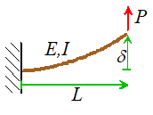
The basic idea is simple, and is best illustrated by
example. Suppose we wish to use FEA to
calculate the deflection of the tip of a cantilever with length L, Young’s modulus E and area moment of inertia I,
which is subjected to a force P. We would set this up as an FEA problem,
entering data for L, E, I,
and P in the code, and computing . We could express the functional relationship
as
 If we were asked to calculate the function f numerically, we would have to run
simulations where we vary E, I, L and P independently. This would be very painful. Fortunately, since the
relationship must be independent of the system of units, we know we can
re-write this expression so that both left and right hand side are dimensionless i.e. as combinations of variables that have no units. Noting that and L
have dimensions of length, I has
dimensions of ,
P has dimensions and E has
dimensions of ,
we could put
If we were asked to calculate the function f numerically, we would have to run
simulations where we vary E, I, L and P independently. This would be very painful. Fortunately, since the
relationship must be independent of the system of units, we know we can
re-write this expression so that both left and right hand side are dimensionless i.e. as combinations of variables that have no units. Noting that and L
have dimensions of length, I has
dimensions of ,
P has dimensions and E has
dimensions of ,
we could put
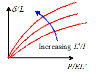
Now, we only need to calculate the function g.
We could do this by keeping L
and I fixed, and varying P to see the results of varying the
first group; we could then keep P and
L fixed and vary I to see the effect of varying the second group. The results could be displayed graphically as
shown in the figure.
If we had done a linear
analysis (no nonlinear geometric effects) the curves would be straight lines.
There is often more than one choice of dimensionless
group, and some are better than others.
For example, for the beam problem we could create a new dimensionless
group by multiplying together the two groups in the function g this gives
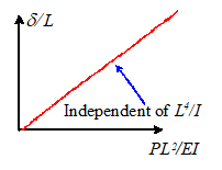
This turns out to be a much better choice. In fact, if
we conducted a linear analysis we would find that the function h is independent
of . In this case the data would collapse onto a
single master-curve as shown in the figure.
Unfortunately, dimensional analysis alone will not
tell you the best dimensionless groups.
You have to use your physical intuition to identify them. For the beam example, you might remember that
E and I always appear as the product EI
in the governing equations so it makes sense to try to find dimensionless
groups that combine them in this way.
In other examples, you may see some physical significance of
combinations of variables (they might look like a kinetic energy, or a
pressure, for example) which might help you to choose the best set.
The beauty of using dimensional analysis to simplify
numerical simulations is that, unlike in experiments, you don’t need to guess
what variables influence the results.
You know exactly what they are, because you typed them into the program!
The following steps (known as the Buckingham Pi
theorem) will tell you how many dimensionless groups to look for:
1. List the variable you are computing, and also the
variables you entered into the code to define the problem. Count the total number of variables and call
it n
2. List the dimensions, in terms of fundamental units
(i.e. mass, length, time, electric current, and luminous intensity) of all the
variables
3. Count the number of independent fundamental units that appear in the problem (e.g. if
mass, length and time appear independently, then there are 3 different units)
and call the number k. Units are independent if they don’t always
appear in the same combination. For
example, in our beam problem mass and time are not independent, because they appear together as in both P
and E. The beam problem has length, and as two independent combinations of fundamental
units.
4. A total of n-k
independent dimensionless groups must appear in the dimensionless relationship.
For the beam problem, we had 5 variables ,
and two independent combinations of fundamental units, so we expect to see
three dimensionless groups which is precisely what we got.
Simplifying
FEA analysis by scaling the
governing equations
 An alternative approach to identifying the
dimensionless parameters that control the solution to a problem is to express
the governing equations themselves in dimensionless form. This is a much more powerful technique, but
is also somewhat more difficult to use.
An alternative approach to identifying the
dimensionless parameters that control the solution to a problem is to express
the governing equations themselves in dimensionless form. This is a much more powerful technique, but
is also somewhat more difficult to use.
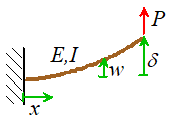
We can illustrate the procedure using our beam problem
again. Let x measure distance along the beam, and let w denote its vertical deflection.
You may remember that linear Euler-Bernoulli beam theory gives the
following governing equation for w
(the
right hand side vanishes because no forces act on 0<x<L)
while the boundary conditions are
(If you don’t remember these it doesn’t matter it’s the scaling discussed below that’s
important).
We now re-write the equations so that they are
dimensionless. We aways start by
replacing all field variables (in this case w
and x) with dimensionless
quantities. In this case we could use .
Substituting gives
We now look and see if we can make further
simplifications. Our objective is to
remove as many material and geometric parameters from the equations as
possible, by defining new dimensionless field variables or introducing
dimensionless combinations of material or geometric variables. In this case, we see that if we define a new
dimensionless displacement W so that
substitute, and cancel as many terms as possible, the
governing equations become
In this form, the governing equations contain
absolutely no material or geometric parameters.
The solution for W must
therefore be independent of L,E,I or P.
We can solve the equation just once, and then work out the tip
deflection from the value of W at . Specifically,
This scaling procedure is the best way to simplify
numerical computations. It is more
difficult to apply than dimensional analysis, however, and it is possible
(although perhaps not a good idea) to run an FEA simulation of a problem where
you don’t actually know the governing equations! In this case you should just
use standard dimensional analysis to try to simplify the problem.