Chapter 4

 

Mathematical description of shape changes in solids

 

 

 

In this section, we list the various mathematical formulas that are used to characterize shape changes in solids (and in fluids).  The formulas might look scary at first, but they are mostly just definitions. 

 

As you work through the various definitions, you should bear in mind that shape changes near a point can always be characterized by six numbers.  These could be could be the six independent components of the Lagrangian strain, Eulerian strain, the left or right stretch tensors, or your own favorite deformation measure.  Given the complete set of six numbers for any one deformation measure, you can always calculate the components of other strain measures. The reason that so many different deformation measures exist is partly that different material models adopt different strain measures, and partly because each measure is useful for describing a particular type of shape change.

 

4.1 The Displacement and Velocity Fields

 

The displacement vector u(x,t) describes the motion of each point in the solid. To make this precise, visualize a solid deforming under external loads.  Every point in the solid moves as the load is applied: for example, a point at position x in the undeformed solid might move to a new position y at time t.  The displacement vector is defined as

$y=x+u(x,t)$

We could also express this formula using index notation, as

$y_i=x_i+u_i(x_1,x_2,x_3,t)$

Here, the subscript i  has  values 1,2, or 3, and (for example) $y_i$ represents the three Cartesian components of the vector y.

 

The displacement field completely specifies the change in shape of the solid. The velocity field would describe its motion, as

$v_i(x_k,t)=\frac{\partial y_i}{\partial t}={\frac{\partial u_i(x_k,t)}{\partial t}|}_{x_k=\text{const}}$

 

 

 

 

 

 

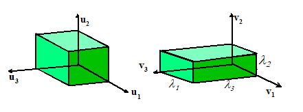
Examples of some simple deformations

 

 

 

 

4.2 The Displacement gradient and Deformation gradient tensors

 

These quantities are defined by

 Displacement Gradient Tensor:   $\nabla u$ is a tensor with components $\frac{\partial u_i}{\partial x_k}$

$$ Deformation Gradient Tensor: $F=I+\nabla u\text{or in Cartesian components }{F}_{ik}={\delta }_{ik}+\frac{\partial u_i}{\partial x_k}$

where I  is the identity tensor, with components described by the Kronekor delta symbol:

${\delta }_{ik}=\{\begin{array}{l}1,i=k\\ 0,i\ne k\end{array}$

and $\nabla$ represents the gradient operator. Formally, the gradient of a vector field u(x) is defined so that

$\left[\nabla u\right]\cdot n=\underset{\alpha \to \text{0}}{\text{Lim}}\frac{u(x+\alpha n)-u(x)}{\alpha }$

but in practice the component formula $\partial u_i/\partial x_j$ is more useful.

 

Note also that

$\begin{array}{c}\nabla y=\nabla \left(x+u(x)\right)=F\\ \text{or }\frac{\partial y_i}{\partial x_j}=\frac{\partial }{\partial x_j}\left(x_i+u_i\right)={\delta }_{ij}+\frac{\partial u_i}{\partial x_j}=F_{ij}\end{array}$

 

 

 

 

 

 

 

 

The concepts of displacement gradient and deformation gradient are introduced to quantify the change in shape of infinitesimal line elements in a solid body. To see this, imagine drawing a straight line on the undeformed configuration of a solid, as shown in the figure.  The line would be mapped to a smooth curve on the deformed configuration.  However, suppose we focus attention on a line segment dx, much shorter than the radius of curvature of this curve, as shown.  The segment would be straight in the undeformed configuration, and would also be (almost) straight in the deformed configuration.  Thus, no matter how complex a deformation we impose on a solid, infinitesimal line segments are merely stretched and rotated by a deformation.The infinitesimal line segments dx and dy are related by

$dy=F\cdot dx\text{or }d{y}_i=F_{ik}d{x}_k$

Written out as a matrix equation, we have

$\left[\begin{array}{c}d{y}_1\\ d{y}_2\\ d{y}_3\end{array}\right]=\left[\begin{array}{ccc}1+\frac{\partial u_1}{\partial x_1}& \frac{\partial u_1}{\partial x_2}& \frac{\partial u_1}{\partial x_3}\\ \frac{\partial u_2}{\partial x_1}& 1+\frac{\partial u_2}{\partial x_2}& \frac{\partial u_2}{\partial x_3}\\ \frac{\partial u_3}{\partial x_1}& \frac{\partial u_3}{\partial x_2}& 1+\frac{\partial u_3}{\partial x_3}\end{array}\right]\left[\begin{array}{c}d{x}_1\\ d{x}_2\\ d{x}_3\end{array}\right]$

 

To derive this result, consider an infinitesimal line element dx in a deforming solid.  When the solid is deformed, this line element is stretched and rotated to a deformed line element dy.  If we know the displacement field in the solid, we can compute dy=[x+dx+u(x+dx)]-[x+u(x)] from the position vectors of its two end points

$d{y}_i=x_i+d{x}_i+u_i(x_k+d{x}_k)-(x_i+u_i(x_k))$

Expand $u_i(x_k+d{x}_k)$ as a Taylor series

$u_i(x_k+d{x}_k)\approx u_i(x_k)+\frac{\partial u_i}{\partial x_k}d{x}_k$

so that

$d{y}_i=d{x}_i+\frac{\partial u_i}{\partial x_k}d{x}_k=\left({\delta }_{ik}+\frac{\partial u_i}{\partial x_k}\right)d{x}_k$

We identify the term in parentheses as the deformation gradient, so

$d{y}_i=F_{ik}d{x}_k$

 

The inverse of the deformation gradient $F^{-1}$ arises in many calculations.  It is defined through

$d{x}_i=F_{ik}^{-1}d{y}_k$

or alternatively

$F_{ij}^{-1}=\frac{\partial x_i}{\partial y_j}$

 

 

 

4.3 Deformation gradient resulting from two successive deformations

 

Suppose that two successive deformations are applied to a solid, as shown.  Let

$dy=F^{(1)}\cdot dxdz=F^{(2)}\cdot dy\text{or}d{y}_i=F_{ij}^{(1)}d{x}_{j}d{z}_i=F_{ij}^{(2)}d{y}_j$

map infinitesimal line elements from the original configuration to the first deformed shape, and from the first deformed shape to the second, respectively, with

$F^{(1)}={\nabla }_{x}y{F}^{(2)}={\nabla }_{y}z\text{or}{F}_{ij}^{(1)}=\frac{\partial y_i}{\partial x_j}{F}_{ij}^{(2)}=\frac{\partial z_i}{\partial y_j}$

The deformation gradient that maps infinitesimal line elements from the original configuration directly to the second deformed shape then follows as

$dz=F\cdot dx\text{with }F=F^{(2)}\cdot F^{(1)}\text{or}d{z}_i=F_{ij}d{x}_j{F}_{ij}=F_{ik}^{(2)}{F}_{kj}^{(1)}$

Thus, the cumulative deformation gradient due to two successive deformations follows by multiplying their individual deformation gradients.

 

To see this, write the cumulative mapping as $z_i\left(y_j(x_k)\right)$ and apply the chain rule

$d{z}_i=\frac{\partial z_i}{\partial y_j}\frac{\partial y_j}{\partial x_k}d{x}_k$

 

 

 

4.4 The Jacobian of the deformation gradient

 

The Jacobian is defined as

$J=\det \left(F\right)=\det \left({\delta }_{ij}+\frac{\partial u_i}{\partial x_j}\right)$

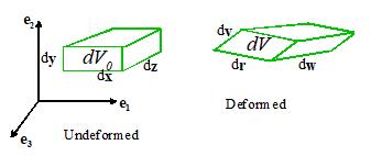
It is a measure of the volume change produced by a deformation.  To see this, consider the infinitessimal volume element shown with sides dx, dy, and dz in the figure above. The original volume of the element is

$d{V}_0=dz\cdot (dx\times dy)={\in }_{ijk}d{z}_{i}d{x}_{j}d{y}_k$

Here,  is the permutation symbol. The element is mapped to a paralellepiped with sides dr, dv, and dw with volume given by

$dV={\in }_{ijk}d{w}_{i}d{r}_{j}d{v}_k$

Recall that

$d{r}_i=F_{il}d{x}_l,d{v}_j=F_{jm}d{y}_m,d{w}_k=F_{kn}d{z}_n$

so that

$dV={\in }_{ijk}{F}_{il}d{x}_l{F}_{jm}d{y}_m{F}_{kn}d{z}_n={\in }_{ijk}{F}_{il}{F}_{jm}{F}_{kn}d{x}_{l}d{y}_{m}d{z}_n$

Recall that

${\in }_{ijk}{A}_{il}{A}_{jm}{A}_{kn}={\in }_{lmn}\det (A)$

so that

$dV=\det (F){\in }_{lmn}d{x}_{l}d{y}_{m}d{z}_n=\det \left(F\right)d{V}_0$

Hence

$\frac{dV}{d{V}_0}=\det \left(F\right)=J$

Observe that

 For any physically admissible deformation, the volume of the deformed element must be positive (no matter how much you deform a solid, you can’t make material disappear).  Therefore, all physically admissible displacement fields must satisfy J>0

 If a material is incompressible, its volume remains constant.  This requires J=1.

 If the mass density of the material at a point in the undeformed solid is ${\rho }_0$, its mass density in the deformed solid is $\rho ={\rho }_0/J$

 

Derivatives of J. When working with constitutive equations, it is occasionally necessary to evaluate derivatives of J with respect to the components of F.  The following result (which can be proved e.g. by expanding the Jacobian using index notation) is extremely useful

$\frac{\partial J}{\partial F_{ij}}=J{F}_{ji}^{-1}$

 

4.5 The Lagrange strain tensor

 

The Lagrange strain tensor is defined as

$E=\frac{1}{2}(F^T\cdot F-I)\text{or}{E}_{ij}=\frac{1}{2}(F_{ki}{F}_{kj}-{\delta }_{ij})$

The components of Lagrange strain can also be expressed in terms of the displacement gradient as

$E_{ij}=\frac{1}{2}\left(\frac{\partial u_i}{\partial x_j}+\frac{\partial u_j}{\partial x_i}+\frac{\partial u_k}{\partial x_j}\frac{\partial u_k}{\partial x_i}\right)$

 

The Lagrange strain tensor quantifies the changes in length of a material fiber, and angles between pairs of fibers in a deformable solid.  It is used in calculations where large shape changes are expected.

 

To visualize the physical significance of E, suppose we mark out an imaginary tensile specimen with (very short) length  on our deforming solid, as shown in the picture. The orientation of the specimen is arbitrary, and is specified by a unit vector m, with components $m_i$.  Upon deformation, the specimen increases in length to $l=l_0+\delta l$. Define the strain of the specimen as

${\epsilon }_L(m_i)=\frac{l^2-l_0{}^2}{2l_0{}^2}=\frac{\delta l}{l_0}+\frac{{\left(\delta l\right)}^2}{2l_0^2}$

Note that this definition of strain is similar to the definition $\epsilon =\delta l/l_0$ you are familiar with, but contains an additional term.  The additional term is negligible for small $\delta l$. Given the Lagrange strain components $E_{ij}$, the strain of the specimen may be computed from

${\epsilon }_L(m)=m\cdot E\cdot m\text{or }{\epsilon }_L(m_i)=E_{ij}{m}_i{m}_j$

We proceed to derive this result. Note that

$d{x}_i=l_0{m}_i$

is an infinitesimal vector with length and orientation of our undeformed specimen.  From the preceding section, this vector is stretched and rotated to

$d{y}_k=\left({\delta }_{kj}+\frac{\partial u_k}{\partial x_j}\right)d{x}_j=\left({\delta }_{kj}+\frac{\partial u_k}{\partial x_j}\right)l_0{m}_j$

The length of the deformed specimen is equal to the length of  dy, so we see that

$\begin{array}{l}{l}^2=d{y}_{k}d{y}_k=\left({\delta }_{kj}+\frac{\partial u_k}{\partial x_j}\right)l_0{m}_j\left({\delta }_{ki}+\frac{\partial u_k}{\partial x_i}\right)l_0{m}_i\\ =\left({\delta }_{ij}+\frac{\partial u_i}{\partial x_j}+\frac{\partial u_j}{\partial x_i}+\frac{\partial u_k}{\partial x_i}\frac{\partial u_k}{\partial x_j}\right)l_0{}^2{m}_j{m}_i\end{array}$

Hence,  the strain for our line element is

${\epsilon }_L(m_i)=\frac{l^2-l_0{}^2}{2l_0{}^2}=\frac{1}{2}\left(\frac{\partial u_i}{\partial x_j}+\frac{\partial u_j}{\partial x_i}+\frac{\partial u_k}{\partial x_j}\frac{\partial u_k}{\partial x_i}\right)m_i{m}_j$

giving the results stated.

 

 

Example 1: Calculate the deformation gradient and Lagrange strain tensor for a volume preserving uniaxial deformation described by the mapping

$\begin{array}{l}{y}_1=\lambda x_1\\ y_2=x_2/\sqrt{\lambda }\\ y_3=x_3/\sqrt{\lambda }\end{array}$

Check that the mapping does preserve volume.

 

This is just a matter of substituting into the formulas

$\begin{array}{l}{F}_{ij}=\frac{\partial y_i}{\partial x_j}\Rightarrow F_{11}=\lambda F_{22}=F_{33}=\frac{1}{\sqrt{\lambda }}\text{all other }{F}_{ij}=0\\ \Rightarrow F=\left[\begin{array}{ccc}\lambda & 0& 0\\ 0& 1/\sqrt{\lambda }& 0\\ 0& 0& 1/\sqrt{\lambda }\end{array}\right]\end{array}$

 

Hence

$E=\frac{1}{2}(F^T\cdot F-I)=\frac{1}{2}\left[\begin{array}{ccc}{\lambda }^2-1& 0& 0\\ 0& 1/\lambda -1& 0\\ 0& 0& 1/\lambda -1\end{array}\right]$

You can see that det(F)=1, so the mapping is volume preserving

 

                                               

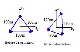Example 2:  To track the deformation in a slowly moving glacier, three survey stations are installed in the shape of an equilateral triangle, spaced 100m apart, as shown in the picture.  After a suitable period of time, the spacing between the three stations is measured again, and found to be 90m, 110m and 120m, as shown in the figure.  Assuming that the deformation of the glacier is homogeneous over the region spanned by the survey stations, please compute the components of the Lagrange strain tensor associated with this deformation, expressing your answer as components in the basis shown.

 

Recall that the initial and deformed lengths $l,l_0$ of a material element parallel to a unit vector $m$ in the undeformed configuration are related by

$\frac{l^2-l_0^2}{2l_0^2}=E_{ij}{m}_i{m}_j=m\cdot Em$

The three unit vectors parallel to the sides of the triangle are $(1,0,0)(1/2,\sqrt{3}/2,0)(-1/2,\sqrt{3}/2,0)$.   Multiplying out the vectors for the three sides of the triangle gives

$\begin{array}{l}\frac{{90}^2-{100}^2}{{2.100}^2}=\left[\begin{array}{cc}1& 0\end{array}\right]\left[\begin{array}{cc}{E}_{11}& E_{12}\\ E_{12}& E_{22}\end{array}\right]\left[\begin{array}{c}0\\ 1\end{array}\right]\frac{{110}^2-{100}^2}{{2.100}^2}=\left[\begin{array}{cc}1/2& \sqrt{3}/2\end{array}\right]\left[\begin{array}{cc}{E}_{11}& E_{12}\\ E_{12}& E_{22}\end{array}\right]\left[\begin{array}{c}1/2\\ \sqrt{3}/2\end{array}\right]\\ \frac{{120}^2-{100}^2}{{2.100}^2}=\left[\begin{array}{cc}-1/2& \sqrt{3}/2\end{array}\right]\left[\begin{array}{cc}{E}_{11}& E_{12}\\ E_{12}& E_{22}\end{array}\right]\left[\begin{array}{c}-1/2\\ \sqrt{3}/2\end{array}\right]\\ \Rightarrow \frac{{90}^2-{100}^2}{{2.100}^2}=E_{11}\frac{{110}^2-{100}^2}{{2.100}^2}=\frac{E_{11}}{4}+\frac{3E_{22}}{4}-\frac{E_{12}\sqrt{3}}{2}\\ \frac{{120}^2-{100}^2}{{2.100}^2}=\frac{E_{11}}{4}+\frac{3E_{22}}{4}+\frac{E_{12}\sqrt{3}}{2}\end{array}$

These three equations can be solved for the Lagrange strain components, with the result

$E_{11}=-19/200E_{22}=149/600E_{12}=23\sqrt{3}/600$ or $E_{11}=-0.095E_{22}=0.2483E_{12}=0.0664$

 

 

 

 

 

4.6 The Infinitesimal strain tensor

 

The infinitesimal strain tensor is defined as

$\epsilon =\frac{1}{2}\left(\nabla u+{\left(\nabla u\right)}^T\right)\text{or }{\epsilon }_{ij}=\frac{1}{2}\left(\frac{\partial u_i}{\partial x_j}+\frac{\partial u_j}{\partial x_i}\right)$

where u is the displacement vector.  Written out in full

${\epsilon }_{ij}\equiv \left[\begin{array}{ccc}\frac{\partial u_1}{\partial x_1}& \frac{1}{2}\left(\frac{\partial u_1}{\partial x_2}+\frac{\partial u_2}{\partial x_1}\right)& \frac{1}{2}\left(\frac{\partial u_1}{\partial x_3}+\frac{\partial u_3}{\partial x_1}\right)\\ \frac{1}{2}\left(\frac{\partial u_2}{\partial x_1}+\frac{\partial u_1}{\partial x_2}\right)& \frac{\partial u_2}{\partial x_2}& \frac{1}{2}\left(\frac{\partial u_2}{\partial x_3}+\frac{\partial u_3}{\partial x_2}\right)\\ \frac{1}{2}\left(\frac{\partial u_3}{\partial x_1}+\frac{\partial u_1}{\partial x_3}\right)& \frac{1}{2}\left(\frac{\partial u_3}{\partial x_2}+\frac{\partial u_2}{\partial x_3}\right)& \frac{\partial u_3}{\partial x_3}\end{array}\right]$

 

The infinitesimal strain tensor is an approximate deformation measure, which is only valid for small shape changes.  It is more convenient than the Lagrange or Eulerian strain, because it is linear.

 

Specifically, suppose the deformation gradients are small, so that all $\partial u_i/\partial x_j<<1$. Then the Lagrange strain tensor is

$E_{ij}=\frac{1}{2}\left(\frac{\partial u_i}{\partial x_j}+\frac{\partial u_j}{\partial x_i}+\frac{\partial u_k}{\partial x_j}\frac{\partial u_k}{\partial x_i}\right)\approx \frac{1}{2}\left(\frac{\partial u_i}{\partial x_j}+\frac{\partial u_j}{\partial x_i}\right)\approx {\epsilon }_{ij}$

so the infinitesimal strain approximates the Lagrange strain.  You can show that it also approximates the Eulerian strain with the same accuracy.

 

Properties of the infinitesimal strain tensor

 

 For small strains, the engineering strain of an infinitesimal fiber aligned with a unit vector m can be estimated as

${\epsilon }_e(m)=\frac{l-l_0}{l_0}\approx {\epsilon }_{ij}{m}_i{m}_j$

 Note that

$\text{trace}\left(\epsilon \right)\equiv {\epsilon }_{kk}=\frac{\partial u_1}{\partial x_1}+\frac{\partial u_2}{\partial x_2}+\frac{\partial u_3}{\partial x_3}=\frac{dV-d{V}_0}{d{V}_0}$

 (see below for more details)

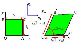
 The infinitesimal strain tensor is closely related to the strain matrix introduced in elementary strength of materials courses.  For example, the physical significance of the (2 dimensional) strain matrix

$\left[\begin{array}{cc}{\epsilon }_{xx}& {\gamma }_{xy}\\ {\gamma }_{yx}& {\epsilon }_{yy}\end{array}\right]$

is illustrated in the figure.

 

To relate this to the infintesimal strain tensor, let $\{e_1,e_2,e_3\}$ be a Cartesian basis, with $e_1$ parallel to x and $e_2$ parallel to y as shown.  Let ${\epsilon }_{ij}$ denote the components of the infinitesimal strain tensor in this basis.  Then

$\begin{array}{l}{\epsilon }_{11}={\epsilon }_{xx}\\ {\epsilon }_{22}={\epsilon }_{yy}\\ {\epsilon }_{12}={\epsilon }_{21}={\gamma }_{xy}/2={\gamma }_{yx}/2\end{array}$

 

 

4.7 Engineering shear strains

 

For a general strain tensor (which could be any of $E$, $E^{*}$ or $\epsilon$, among others), the diagonal strain components ${\epsilon }_{11},{\epsilon }_{22},{\epsilon }_{33}$ are known as `direct’ strains, while the off diagonal terms  ${\epsilon }_{12}={\epsilon }_{21}{\epsilon }_{13}={\epsilon }_{31}{\epsilon }_{23}={\epsilon }_{32}$ are known as ‘shear strains’

 

The shear strains are sometimes reported as ‘Engineering Shear Strains’ which are related to the formal definition by a factor of 2 i.e.

${\gamma }_{12}=2{\epsilon }_{12}{\gamma }_{13}=2{\epsilon }_{13}{\gamma }_{23}=2{\epsilon }_{23}$

 

This factor of 2 is an endless source of confusion.  Whenever someone reports shear strain to you, be sure to check which definition they are using.  In particular, many commercial finite element codes output engineering shear strains.

 

 

4.8 Decomposition of infinitesimal strain into volumetric and deviatoric parts

 

The volumetric infinitesimal strain is defined as $\text{trace(}\epsilon )\equiv {\epsilon }_{kk}$

The deviatoric infinitesimal strain is defined as $e\text{=}\epsilon -\frac{1}{3}I\text{trace(}\epsilon )\equiv e_{ij}={\epsilon }_{ij}-\frac{1}{3}{\delta }_{ij}{\epsilon }_{kk}$

 

The volumetric strain is a measure of volume changes, and for small strains is related to the Jacobian of the deformation gradient by ${\epsilon }_{kk}\approx J-1$.  To see this, recall that

$J=\det \left[\begin{array}{ccc}1+\frac{\partial u_1}{\partial x_1}& \frac{\partial u_1}{\partial x_2}& \frac{\partial u_1}{\partial x_3}\\ \frac{\partial u_2}{\partial x_1}& 1+\frac{\partial u_2}{\partial x_2}& \frac{\partial u_2}{\partial x_3}\\ \frac{\partial u_3}{\partial x_1}& \frac{\partial u_3}{\partial x_2}& 1+\frac{\partial u_3}{\partial x_3}\end{array}\right]\approx \left(1+\frac{\partial u_1}{\partial x_1}\right)\left(1+\frac{\partial u_2}{\partial x_2}\right)\left(1+\frac{\partial u_3}{\partial x_3}\right)\approx 1+\frac{\partial u_1}{\partial x_1}+\frac{\partial u_2}{\partial x_2}+\frac{\partial u_3}{\partial x_3}$

The deviatioric strain is a measure of shear deformation (shear deformation involves no volume change).

 

 

 

4.9 The Infinitesimal rotation tensor

 

The infinitesimal rotation tensor is defined as

$w=\frac{1}{2}\left(\nabla u-{\left(\nabla u\right)}^T\right)\text{or }{w}_{ij}=\frac{1}{2}\left(\frac{\partial u_i}{\partial x_j}-\frac{\partial u_j}{\partial x_i}\right)$

Written out as a matrix, the components of  are

$w_{ij}\equiv \left[\begin{array}{ccc}0& \frac{1}{2}\left(\frac{\partial u_1}{\partial x_2}-\frac{\partial u_2}{\partial x_1}\right)& \frac{1}{2}\left(\frac{\partial u_1}{\partial x_3}-\frac{\partial u_3}{\partial x_1}\right)\\ \frac{1}{2}\left(\frac{\partial u_2}{\partial x_1}-\frac{\partial u_1}{\partial x_2}\right)& 0& \frac{1}{2}\left(\frac{\partial u_2}{\partial x_3}-\frac{\partial u_3}{\partial x_2}\right)\\ \frac{1}{2}\left(\frac{\partial u_3}{\partial x_1}-\frac{\partial u_1}{\partial x_3}\right)& \frac{1}{2}\left(\frac{\partial u_3}{\partial x_2}-\frac{\partial u_2}{\partial x_3}\right)& 0\end{array}\right]$

Observe that $w_{ij}$ is skew symmetric: $w_{ij}=-w_{ji}$. 

 

A skew tensor represents a rotation through a small angle.  Specifically, the operation .. rotates the infinitesimal line element $d{x}_j$ through a small angle $\theta =\sqrt{w_{ij}{w}_{ij}/2}$ about an axis parallel to the unit vector $n_i={\in }_{ijk}{w}_{kj}/(2\theta )$.  (A skew tensor also sometimes represents an angular velocity). 

To visualize the significance of  $w_{ij}$, consider the behavior of an imaginary, infinitesimal, tensile specimen embedded in a deforming solid.  The specimen is stretched, and then rotated through an angle $\varphi$ about some axis q.  If the displacement gradients are small, then $\varphi <<1$.

 

The rotation of the specimen depends on its original orientation, represented by the unit vector m.  One can show (although one would rather not do all the algebra) that $w_{ij}$ represents the average rotation, over all possible orientations of m, of material fibers passing through a point.

 

As a final remark, we note that a general deformation can always be decomposed into an infinitesimal strain and rotation

$\frac{\partial u_i}{\partial x_j}=\frac{1}{2}\left(\frac{\partial u_i}{\partial x_j}+\frac{\partial u_j}{\partial x_i}\right)+\frac{1}{2}\left(\frac{\partial u_i}{\partial x_j}-\frac{\partial u_j}{\partial x_i}\right)={\epsilon }_{ij}+w_{ij}$

Physically, this sum of ${\epsilon }_{ij}$ and $w_{ij}$ can be regarded as representing two successive deformations $–$ a small strain, followed by a rotation, in the sense that

$d{y}_i=\left({\delta }_{ik}+w_{ik}\right)\left({\delta }_{kj}+{\epsilon }_{kj}\right)d{x}_j\approx d{x}_i+\left({\epsilon }_{ij}+w_{ij}\right)d{x}_j$

first stretches the infinitesimal line element, then rotates it.

 

4.10 Principal values and directions of the infinitesimal strain tensor

The three principal values $e_i$ and directions $n^{(i)}$ of the infinitesimal strain tensor satisfy

$\begin{array}{c}\epsilon \cdot n^{(i)}=e_i{n}^{(i)}\\ \text{or }{\epsilon }_{kl}{n}_l^{(i)}=e_i{n}_l^{(i)}\end{array}$

Clearly, $e_i$ and $n^{(i)}$ are the eigenvalues and eigenvectors of $\epsilon$.  There are three principal strains and three principal directions, which are always mutually perpendicular. 

 

Their significance can be visualized as follows.

1.      Note that the decomposition $\frac{\partial u_i}{\partial x_j}={\epsilon }_{ij}+w_{ij}$ can be visualized as a small strain, followed by a small rigid rotation, as shown in the picture.

2.      The formula $\epsilon \cdot n^{(i)}=e_i{n}^{(i)}$ indicates that a vector n is mapped to another, parallel vector by the strain.

3.      Thus, if you draw a small cube with its faces perpendicular to $n^{(i)}$ on the undeformed solid, this cube will be stretched perpendicular to each face, with a fractional increase in length $e_i=\delta l_i/l_0$.  The faces remain perpendicular to $n^{(i)}$ after deformation.

4.      Finally, w rotates the small cube through a small angle onto its configuration in the deformed solid.

 

 

Example: The twisted cylinder shown in the figure has a displacement field (in polar coordinates)

$u=\frac{\varphi }{L}rz{e}_{\theta }$

 

where $\varphi$ is the angle of twist at the end of the cylinder.  The contours show the magnitude of the displacement vector, to help visualize the deformation.

 

(a) Calculate the infinitesimal strain tensor in the cylinder.  Hence determine the engineering shear strains

 

We need the cylindrical-polar formulas for the gradient of a vector v from Section 3.6 of the notes

 

 

$\nabla v\equiv \left[\begin{array}{ccc}\frac{\partial v_r}{\partial r}& \frac{1}{r}\frac{\partial v_r}{\partial \theta }-\frac{v_{\theta }}{r}& \frac{\partial v_r}{\partial z}\\ \frac{\partial v_{\theta }}{\partial r}& \frac{1}{r}\frac{\partial v_{\theta }}{\partial \theta }+\frac{v_r}{r}& \frac{\partial v_{\theta }}{\partial z}\\ \frac{\partial v_z}{\partial r}& \frac{1}{r}\frac{\partial v_z}{\partial \theta }& \frac{\partial v_z}{\partial z}\end{array}\right]$

 

In the problem here $u_{\theta }=\varphi rz/L$ and all the other displacement components are zero.  Therefore

$\nabla u\equiv \left[\begin{array}{ccc}0& -\frac{\varphi z}{L}& 0\\ \frac{\varphi z}{L}& 0& \frac{\varphi r}{L}\\ 0& 0& 0\end{array}\right]$

 

The infinitesimal strain tensor follows as

$\frac{1}{2}\left(\nabla u+{\left(\nabla u\right)}^T\right)\equiv \left[\begin{array}{ccc}0& 0& 0\\ 0& 0& \frac{\varphi r}{2L}\\ 0& \frac{\varphi r}{2L}& 0\end{array}\right]$

 

The engineering shear strains (which you may remember from intro courses) is ${\gamma }_{rz}={\gamma }_{zr}=\varphi r/L$ .  Note the factor of 2.

 

(b) Calculate the Lagrange strain tensor in the bar.   Find a formula for the difference between the infinitesimal strain and the Lagrange strain.

 

It gets a bit tedious to do these problems by hand so here is a Matlab Live Script solution

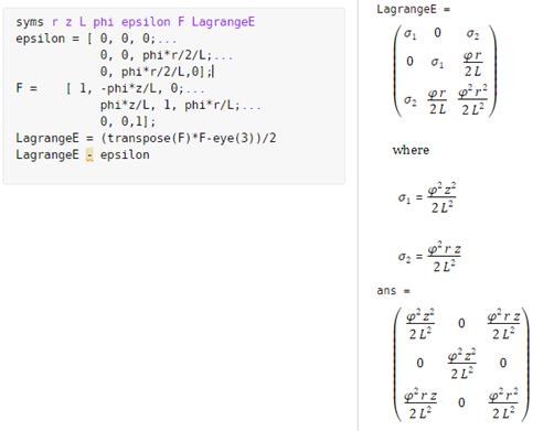
Note that as long as the twist angle is small, the infinitesimal strain is approximately equal to the Lagrange strain.

 

(c) Calculate the principal strains and the directions of the principal strains

 

More Live Scripts

 

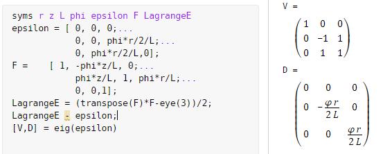
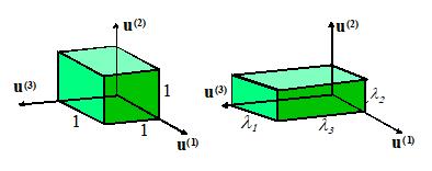
The matrix V contains the three eigenvectors as columns (they are not unit vectors).  The matrix D contains the principal strain values on the diagonals.  The principal strain directions are therefore at 45 degrees to the $e_z,e_{\theta }$ directions.   The deformation of a square element is illustrated in the figure below.  The volume is constant; and the element is stretched parallel to one principal direction, and compressed parallel to the other.

 

 

 

 

 

4.11 Cauchy-Green Deformation Tensors

 

The Cauchy-Green deformation tensors are used to model highly deformable solids such as rubbers or tissue.   They are defined through

 The Right Cauchy Green Deformation Tensor   $C=F^T\cdot F{C}_{ij}=F_{ki}{F}_{kj}$

 The Left Cauchy Green Deformation Tensor     $B=F\cdot F^T{B}_{ij}=F_{ik}{F}_{jk}$

They are called `left’ and `right’ tensors because of their relation to the `left’ and ‘right’ stretch tensors defined below.  They can be regarded as quantifying the squared length of infinitesimal fibers in the deformed configuration, by noting that if a material fiber $dx=l_{0}m$ in the undeformed solid is stretched and rotated to $dy=ln$ in the deformed solid, then

$\frac{l^2}{l_0^2}=m\cdot C\cdot m\frac{l_0^2}{l^2}=n\cdot B^{-1}\cdot n$

 

 

 

 

 

 

 

4.12  Rotation tensor, and Left and Right Stretch Tensors

 

The definitions of these quantities are

 The Right Stretch Tensor $U=C^{1/2}={\left(F^T\cdot F\right)}^{1/2}{U}_{ij}=C_{ij}^{1/2}$

 The Left Stretch Tensor   $V=B^{1/2}{V}_{ij}=B_{ij}^{1/2}$

 The Rotation Tensor         $R=F\cdot U^{-1}=V^{-1}\cdot F{R}_{ij}=F_{ik}{U}_{kj}^{-1}=V_{ik}^{-1}{F}_{kj}$

 

To calculate these quantities you need to remember how to calculate the square root of a matrix.  For example, to calculate the square root of C, you must

1.      Calculate the eigenvalues of C $–$ we will call these ${\lambda }_n^2$, with n=1,2,3.  Since C and B are both symmetric and positive definite, the eigenvalues ${\lambda }_n^2$ are all positive real numbers, and therefore their square roots ${\lambda }_n$ are also positive real numbers.

2.      Calculate the eigenvectors of C and normalize them so they have unit magnitude.  We will denote the eigenvectors by $c^{(n)}$.  They must be normalized to satisfy $c^{(n)}\cdot c^{(n)}=1$

3.      Finally, calculate $C^{1/2}={\displaystyle {\sum }_{n=1}^3{\lambda }_n{c}^{(n)}\otimes c^{(n)}}$, where $c$ denotes a dyadic product In components, this can be written $C_{ij}^{1/2}={\displaystyle {\sum }_{n=1}^3{\lambda }_n{c}_i^{(n)}{c}_j^{(n)}}$

4.      As an additional bonus, you can quickly compute the inverse square root (which is needed to find R) as

$C^{-1/2}={\displaystyle {\sum }_{n=1}^3\frac{1}{{\lambda }_n}{c}^{(n)}\otimes c^{(n)}}\text{or }{C}_{ij}^{-1/2}={\displaystyle {\sum }_{n=1}^3\frac{1}{{\lambda }_n}{c}_i^{(n)}{c}_j^{(n)}}$

 

Of course, MATLAB or similar codes will do these operations for you easily.

 

To see the physical significance of these tensors, observe that

1.      The definition of the rotation tensor shows that

$\begin{array}{l}R=F\cdot U^{-1}\iff F=R\cdot U\\ R=V^{-1}\cdot F\iff F=V\cdot R\end{array}$

2.      The multiplicative decomposition of a constant tensor $F=R\cdot U$ can be regarded as a sequence of two homogeneous deformations $–$ U, followed by R.  Similarly, $F=V\cdot R$ is R followed by V.

3.      R is proper orthogonal (it satisfies $R\cdot R^T=R^T\cdot R=I$ and det(R)=1), and therefore represents a rotation.  To see this, note that U is symmetric, and therefore satisfies $U^{-T}=U^{-1}$, so that

$\begin{array}{l}{R}^{T}R={\left(F\cdot U^{-1}\right)}^T\cdot \left(F\cdot U^{-1}\right)\\ =U^{-T}\cdot F^T\cdot F\cdot U^{-1}\\ =U^{-1}\cdot U^2\cdot U^{-1}=I\end{array}$

and det(R)=det(F)det(U^-1)=1

4. U can be expressed in the form

$U={\lambda }_1{u}^{(1)}\otimes u^{(1)}+{\lambda }_2{u}^{(2)}\otimes u^{(2)}+{\lambda }_3{u}^{(3)}\otimes u^{(3)}$

where $u^{(i)}$ are the three (mutually perpendicular) eigenvectors of U. (By construction, these are identical to the eigenvectors of C).  If we interpret $u^{(i)}$ as basis vectors, we see that U is diagonal in this basis, and so corresponds to stretching parallel to each basis vector, as shown in the figure below.

The decompositions

$F=R\cdot U$ and $F=V\cdot R$

are known as the right and left polar decomposition of F. (The right and left refer to the positions of U and V).  They show that every homogeneous deformation can be decomposed into a stretch followed by a rigid rotation, or equivalently into a rigid rotation followed by a stretch. The decomposition is discussed in more detail in the next section.

 

 

4.13 Principal stretches

 

The principal stretches can be calculated from any one of the following (they all give the same answer)

1. The eigenvalues of the right stretch tensor U
2. The eigenvalues of the left stretch tensor V
3. The square root of the eigenvalues of the right Cauchy-Green tensor C
4. The square root of the eigenvalues of the left Cauchy-Green tensor B

The principal stretches are also related to the eigenvalues of the Lagrange and Eulerian strains.  The details are left as an exercise.

 

There are two sets of principal stretch directions, associated with the undeformed and deformed solids.

1. The principal stretch directions in the undeformed solid are the (normalized) eigenvectors of U or C.  Denote these by $u^{(i)}$.
2. The principal stretch directions in the deformed solid are the (normalized) eigenvectors of V or B. Denote these by $v^{(i)}$.

 

To visualize the physical significance of principal stretches and their directions, note that a deformation can be decomposed as $F=R\cdot U$ into a sequence of a stretch followed by a rotation. 

 

Note also that

1. The principal directions $u^{(i)}$ are mutually perpendicular.  You could draw a little cube on the undeformed solid with faces perpendicular to these directions, as shown above.
2. The stretch U will stretch the cube by an amount ${\lambda }_i$ parallel to each $u^{(i)}$.  The faces of the stretched cube remain perpendicular to $u^{(i)}$.
3. The rotation R will rotate the stretched cube so that the directions $u^{(i)}$ rotate to line up with $v^{(i)}$.
4. The faces of the deformed cube are perpendicular to $v^{(i)}$

The decomposition $F=V\cdot R$ can be visualized in much the same way.  In this case, the directions $u^{(i)}$ are first rotated to coincide with $v^{(i)}$.  The cube is then stretched parallel to each $v^{(i)}$ to produce the same shape change.

 

We could compare the undeformed and deformed cubes by placing them side by side, with the vectors $v^{(i)}$ and $u^{(i)}$ parallel, as shown in the figure. 

 

 

Example: a spherical shell (see the figure) is made from an incompressible material.  In its undeformed state, the inner and outer radii of the shell are $A,B$.  After deformation, the new values are $a,b$.  The deformation in the shell can be described (in Cartesian components) by the equation

$y_i=r\frac{x_i}{R}r={\left(R^3+a^3-A^3\right)}^{1/3}R=\sqrt{x_k{x}_k}$

 

(a) Calculate the components of the deformation gradient tensor

 

It is fastest to do this with index notation.   Remember (see the examples at the end of Sect 3.7)

$\frac{\partial x_i}{\partial x_j}={\delta }_{ij}\frac{\partial R}{\partial x_j}=\frac{1}{2}\frac{2{\delta }_{jk}{x}_k}{\sqrt{x_k{x}_k}}=\frac{x_j}{R}$

Hence

 

$\begin{array}{l}{F}_{ij}=\frac{\partial y_i}{\partial x_j}={\left(R^3+a^3-A^3\right)}^{-2/3}{x}_i{x}_j+{\left(R^3+a^3-A^3\right)}^{1/3}\left(\frac{{\delta }_{ij}}{R}-\frac{x_i{x}_j}{R^3}\right)\\ ={\delta }_{ij}\frac{r}{R}+\left(\frac{R^2}{r^2}-\frac{r}{R}\right)\frac{x_i{x}_j}{R^2}\end{array}$

 

(b) Verify that the deformation is volume preserving

 

Since the deformation is radially symmetric, we can compute J along any radial line.  Taking $x_1=R,x_2=x_3=0$, we see that

$F_{11}=\frac{R^2}{r^2}{F}_{22}=F_{33}=\frac{r}{R}\Rightarrow \det (F)=F_{11}{F}_{22}{F}_{33}=1$

(c)  Find the deformed length of an infinitesimal radial line that has initial length $l_0$, expressed as a function of R

 

Let $d{x}_i=l_0\frac{x_i}{R}$.  Then $d{y}_i=F_{ij}d{x}_j=\left({\delta }_{ij}\frac{r}{R}+\left(\frac{R^2}{r^2}-\frac{r}{R}\right)\frac{x_i{x}_j}{R^2}\right)l_0\frac{x_j}{R}=l_0\frac{R^2}{r^2}\frac{x_i}{R}$ and $\sqrt{d{y}_{i}d{y}_i}=l_0\frac{R^2}{r^2}$.

 

(d) Find the deformed length of an infinitesimal circumferential line that has initial length $l_0$, expressed as a function of R

 

Since the deformation is volume preserving, $l_{\theta }^2{l}_r=l_0^3\Rightarrow l_{\theta }=\sqrt{\frac{l_0^3}{l_r}}=l_0\frac{r}{R}$ 

 

(e)  Using the results of (c) and (d), write down the principal stretches for the deformation.

 

If $m_i$ is a principal stretch direction, the principal stretches ${\lambda }_i$ have the property that $l{m}_i={\lambda }_i{l}_0{m}_i$ (no sum on i).   The principal stretch directions are radial and circumferential, by inspection.   From (c) and (d), it follows that ${\lambda }_1=R^2/r^2{\lambda }_2={\lambda }_3=r/R$.

 

 

 

Example:  Repeat problem (a) from above, but this time solve the problem using spherical-polar coordinates, using the various formulas for vector and tensor operations given in Section 3.5 of the notes.   In this case, you may assume that a point with position $x=R{e}_R$ in the undeformed solid has position vector

$y={\left(R^3+a^3-A^3\right)}^{1/3}{e}_R$

after deformation.

 

 

 

We need the following result from Section 3.5:  the gradient of a vector with components $v_R,v_{\theta },v_{\varphi }$ is

$\nabla v\equiv \left[\begin{array}{ccc}\frac{\partial v_R}{\partial R}& \frac{1}{R}\frac{\partial v_R}{\partial \theta }-\frac{v_{\theta }}{R}& \frac{1}{R\sin \theta }\frac{\partial v_R}{\partial \varphi }-\frac{v_{\varphi }}{R}\\ \frac{\partial v_{\theta }}{\partial R}& \frac{1}{R}\frac{\partial v_{\theta }}{\partial \theta }+\frac{v_R}{R}& \frac{1}{R\sin \theta }\frac{\partial v_{\theta }}{\partial \varphi }-\cot \theta \frac{v_{\varphi }}{R}\\ \frac{\partial v_{\varphi }}{\partial R}& \frac{1}{R}\frac{\partial v_{\varphi }}{\partial \theta }& \frac{1}{R\sin \theta }\frac{\partial v_{\varphi }}{\partial \varphi }+\cot \theta \frac{v_{\theta }}{R}+\frac{v_R}{R}\end{array}\right]$

For our problem

$v_r={\left(R^3+a^3-A^3\right)}^{1/3}{v}_{\theta }=v_{\varphi }=0$

Hence

 

$F\equiv \left[\begin{array}{ccc}\frac{\partial v_R}{\partial R}& 0& 0\\ 0& \frac{v_R}{R}& 0\\ 0& 0& +\frac{v_R}{R}\end{array}\right]=\left[\begin{array}{ccc}\frac{R^2}{r^2}& 0& 0\\ 0& \frac{r}{R}& 0\\ 0& 0& \frac{r}{R}\end{array}\right]r={(R^3+a^3-A^3)}^{1/3}$

 

 

Alternatively we can do the calculation using the gradient operator

 

 

$\nabla \equiv \left(e_R\frac{\partial }{\partial R}+e_{\theta }\frac{1}{R}\frac{\partial }{\partial \theta }+e_{\varphi }\frac{1}{R\sin \theta }\frac{\partial }{\partial \varphi }\right)$

and the derivatives of the basis vectors are

$\begin{array}{l}\frac{\partial e_R}{\partial R}=\frac{\partial e_{\theta }}{\partial R}=\frac{\partial e_{\varphi }}{\partial R}=0\frac{\partial e_R}{\partial \theta }=e_{\theta }\frac{\partial e_{\theta }}{\partial \theta }=-e_R\frac{\partial e_{\varphi }}{\partial \theta }=0\\ \frac{\partial e_R}{\partial \varphi }=\sin \theta e_{\varphi }\frac{\partial e_{\theta }}{\partial \varphi }=\cos \theta e_{\varphi }\frac{\partial e_{\varphi }}{\partial \varphi }=-\sin \theta e_R-\cos \theta e_{\theta }\end{array}$

Then the deformation gradient is: $F=\nabla (R{e}_R)=\frac{R^2}{r^2}{e}_R\otimes e_R+\frac{r}{R}{e}_{\theta }\otimes e_{\theta }+\frac{r}{R}{e}_{\varphi }\otimes e_{\varphi }$

 

These are far simpler than the Cartesian form $–$ that’s why we use spherical coordinates!

 

 

Example: The figure shows the reference and deformed configurations for a solid.  The out-of-plane dimensions are unchanged.  Points a and b are the positions of points A and B after deformation.  Determine

 

 

(a)  The right stretch tensor U, expressed as components in $e_1,e_2,e_3$.  (A 2x2 matrix is sufficient).

 

The deformed configuration can be reached by a stretch parallel to the two basis vectors, followed by a rotation.  These can be taken to be the two deformations in the decomposition  F=RU

$\left[\begin{array}{cc}2& 0\\ 0& 1/4\end{array}\right]$

 

(b) The rotation tensor R  in the polar decomposition of the deformation gradient F=RU=VR

 

The bar is rotated 45 degrees in the counterclockwise direction.   Using the formula from section 4.1 we know that

 

$R=\left[\begin{array}{cc}\cos (45)& -\sin (45)\\ \sin (45)& \cos (45)\end{array}\right]=\frac{1}{\sqrt{2}}\left[\begin{array}{cc}1& -1\\ 1& 1\end{array}\right]$

 

 (c) The deformation gradient, expressed as components in $m_1,m_2,m_3$.  Try to do this without using the basis-change formulas.

 

The deformation gradient can be decomposed as F=VR, and V has components

$\left[\begin{array}{cc}2& 0\\ 0& 1/4\end{array}\right]$

in $m_1,m_2,m_3$, while R has the same components in both $e_1,e_2,e_3$ and $m_1,m_2,m_3$.   Therefore

$\frac{1}{\sqrt{2}}\left[\begin{array}{cc}2& 0\\ 0& 1/4\end{array}\right]\left[\begin{array}{cc}1& -1\\ 1& 1\end{array}\right]=\frac{1}{\sqrt{2}}\left[\begin{array}{cc}2& -2\\ 1/4& 1/4\end{array}\right]$

 

 

4.14 Generalized strain measures

 

The polar decompositions $F=R\cdot U$ and $F=V\cdot R$ provide a way to define additional strain measures.  Let ${\lambda }_i$ denote the principal stretches, and let $u^{(i)}$ and $v^{(i)}$ denote the normalized eigenvectors of U and V.  Then one could define strain tensors through

$\begin{array}{l}\text{Lagrangian Nominal strain: }{\displaystyle \sum _{\text{i=1}}^{\text{3}}({\lambda }_i-1)u^{(i)}\otimes u^{(i)}}\\ \text{Lagrangian Logarithmic strain: }{\displaystyle \sum _{\text{i=1}}^{\text{3}}\log ({\lambda }_i)u^{(i)}\otimes u^{(i)}}\end{array}$

The correspoinding Eulerian strain measures are

$\begin{array}{l}\text{Eulerian Nominal strain: }{\displaystyle \sum _{\text{i=1}}^{\text{3}}({\lambda }_i-1)v^{(i)}\otimes v^{(i)}}\\ \text{Eulerian Logarithmic strain: }{\displaystyle \sum _{\text{i=1}}^{\text{3}}\log ({\lambda }_i)v^{(i)}\otimes v^{(i)}}\end{array}$

Another strain measure can be defined as

$\text{Green's strain: }{E}_G\text{= }{\displaystyle \sum _{\text{i=1}}^{\text{3}}\frac{1}{2}({\lambda }_i^2-1)v^{(i)}\otimes v^{(i)}}$

This can be computed directly from the deformation gradient as

$E_G\text{= }\frac{\text{1}}{\text{2}}\left(F\cdot F^T-I\right)$

and is very similar to the Lagrangean strain tensor, except that its principal directions are rotated through the rigid rotation R.

 

 

 

4.15 The velocity gradient

 

We now list several measures of the rate of deformation. The velocity gradient is the basic measure of deformation rate, and is defined as

$L={\nabla }_{y}v\equiv L_{ij}=\frac{\partial v_i}{\partial y_j}$

It quantifies the relative velocities of two material particles at positions y and y+dy in the deformed solid, in the sense that

$d{v}_i=v_i(y+dy)-v_i(y)=\frac{\partial v_i}{\partial y_j}d{y}_j$

The velocity gradient can be expressed in terms of the deformation gradient and its time derivative as

${\nabla }_{y}v=\dot{F}\cdot F^{-1}\frac{\partial v_i}{\partial y_j}={\dot{F}}_{ik}{F}_{kj}^{-1}$

To see this, note that

$d{v}_i=\frac{d}{dt}d{y}_i=\frac{d}{dt}\left(F_{ij}d{x}_j\right)={\dot{F}}_{ij}d{x}_j$

and recall that $d{y}_j=F_{ji}d{x}_i\Rightarrow d{x}_j=F_{jk}^{-1}d{y}_k$, so that

$d{v}_i={\dot{F}}_{ij}{F}_{jk}^{-1}d{y}_k$

 

 

 

 

4.16 Stretch rate and spin tensors

 

The stretch rate tensor is defined as $D=\left(L+L^T\right)/2D_{ij}=\left(L_{ij}+L_{ji}\right)/2$

The spin tensor is defined as $W=\left(L-L^T\right)/2W_{ij}=\left(L_{ij}-L_{ji}\right)/2$

 

A general velocity gradient can be decomposed into the sum of stretch rate and spin, as

$L=D+W{L}_{ij}=D_{ij}+W_{ij}$

The stretch rate quantifies the rate of stretching of material fibers in the deformed solid, in the sense that

$\frac{1}{l}\frac{dl}{dt}=n\cdot D\cdot n=n_i{D}_{ij}{n}_j$

is the rate of stretching of a material fiber with length l and orientation n in the deformed solid.  To see this, let $dy=ln$, so that

$\frac{d}{dt}dy=\frac{dl}{dt}n+l\frac{dn}{dt}$

By definition,

$\frac{d}{dt}dy=\frac{d}{dt}\left(F\cdot dx\right)=\dot{F}\cdot dx=\dot{F}\cdot \left(F^{-1}dy\right)=\dot{F}{F}^{-1}\cdot dy=L\cdot dy=(D+W)\cdot ln$

Hence

$(D+W)\cdot ln=\frac{dl}{dt}n+l\frac{dn}{dt}$

Finally, take the dot product of both sides with n, note that since n is a unit vector $dn/dt$ must be perpendicular to n and therefore $n\cdot dn/dt=0$.  Note also that $n\cdot W\cdot n=0$, since W is skew-symmetric.  It is easiest to show this using index notation: $n_i{W}_{ij}{n}_j=n_i(L_{ij}-L_{ji})n_j/2=0$.  Therefore

$n\cdot (D+W)\cdot ln=\frac{dl}{dt}n\cdot n+ln\cdot \frac{dn}{dt}\Rightarrow n\cdot D\cdot ln=\frac{dl}{dt}$

The spin tensor W can be shown to provide a measure of the average angular velocity of all material fibers passing through a material point. 

 

 

 

Example: a spherical shell (see the figure) is made from an incompressible material.  In its undeformed state, the inner and outer radii of the shell are $A,B$.  After deformation, the new values are $a,b$.  The deformation in the shell can be described (in Cartesian components) by the equation

$y_i=r\frac{x_i}{R}r={\left(R^3+a^3-A^3\right)}^{1/3}R=\sqrt{x_k{x}_k}$

 

Recall (see the example in Section 4.13) that the deformation gradient is

$\begin{array}{l}{F}_{ij}=\frac{\partial y_i}{\partial x_j}={\left(R^3+a^3-A^3\right)}^{-2/3}{x}_i{x}_j+{\left(R^3+a^3-A^3\right)}^{1/3}\left({\delta }_{ij}-\frac{x_i{x}_j}{R^3}\right)\\ ={\delta }_{ij}\frac{r}{R}+\left(\frac{R^2}{r^2}-\frac{r}{R}\right)\frac{x_i{x}_j}{R^2}\end{array}$

The inverse of the deformation gradient (challenge $–$ can you show this?) is

$F_{ij}^{-1}={\delta }_{ij}\frac{R}{r}+\left(\frac{r^2}{R^2}-\frac{R}{r}\right)\frac{y_i{y}_j}{r^2}$

 

 

Suppose that the shell is continuously expanding (visualize a balloon being inflated).  The rate of expansion can be characterized by the velocity $v_a=da/dt$ of the surface that lies at R=A in the undeformed cylinder.

 

(a) Calculate the velocity field $v_i=d{y}_i/dt$ in the sphere as a function of $x_i$

 

We have that $y_i=r\frac{x_i}{R}r={\left(R^3+a^3-A^3\right)}^{1/3}R=\sqrt{x_k{x}_k}$

Hence $\frac{\partial y_i}{\partial t}=\frac{\partial r}{\partial t}\frac{x_i}{R}=\frac{a^2{v}_a}{r^2}\frac{x_i}{R}$

 

(b) Calculate the velocity field as a function of $y_i$ 

$v_i=\frac{a^2{v}_a}{r^2}\frac{y_i}{r}$

 

(c) Calculate the time derivative of the deformation gradient tensor

 

${\dot{F}}_{ij}={\delta }_{ij}\frac{v_a{a}^2}{R{r}^2}+\left(-2\frac{v_a{a}^2{R}^2}{r^5}-\frac{v_a{a}^2}{R{r}^2}\right)\frac{x_i{x}_j}{R^2}$

(d) Calculate the components of the velocity gradient $L_{ij}=\frac{\partial v_i}{\partial y_j}$ by differentiating the result of (b)

$\frac{\partial v_i}{\partial y_j}=\frac{a^2{v}_a}{r^3}\left({\delta }_{ij}-3\frac{y_i{y}_j}{r^2}\right)$

(e) Calculate the components of the velocity gradient using the results of (c) and the inverse of the deformation gradient

 

The other approach is to use

$\begin{array}{l}\frac{\partial v_i}{\partial y_j}={\dot{F}}_{ik}{F}_{kj}^{-1}=\frac{v_a{a}^2}{R{r}^2}\left[{\delta }_{ik}-\left(1+2\frac{R^3}{r^3}\right)\frac{y_i{y}_k}{r^2}\right]\left[{\delta }_{kj}\frac{R}{r}+\left(\frac{r^2}{R^2}-\frac{R}{r}\right)\frac{y_k{y}_j}{r^2}\right]\\ =\frac{v_a{a}^2}{r^3}\left[{\delta }_{ik}-\left(1+2\frac{R^3}{r^3}\right)\frac{y_i{y}_k}{r^2}\right]\left[{\delta }_{kj}+\left(\frac{r^3}{R^3}-1\right)\frac{y_k{y}_j}{r^2}\right]\\ =\frac{a^2{v}_a}{r^3}\left({\delta }_{ij}-3\frac{y_i{y}_j}{r^2}\right)\end{array}$

 

(f) Calculate the stretch rate tensor $D_{ij}$.  Verify that the result represents a volume preserving stretch rate field.

 

 The stretch rate is the symmetric part of $\frac{\partial v_i}{\partial y_j}$ - but it is symmetric anyway.   So

$D_{ij}=\frac{a^2{v}_a}{r^3}\left({\delta }_{ij}-3\frac{y_i{y}_j}{r^2}\right)$

 

To be volume preserving, $D_{kk}=0$.  It is easy to show that this is indeed satisfied.

 

 

 

 

 

 

4.17 Infinitesimal strain rate and rotation rate

 

For small strains the rate of deformation tensor can be approximated by the infinitesimal strain rate, while the spin can be approximated by the time derivative of the infinitesimal rotation tensor

$\begin{array}{l}\frac{d}{dt}\epsilon =\frac{d}{dt}\frac{1}{2}\left(\nabla u+{\left(\nabla u\right)}^T\right)\approx D\text{or }{\dot{\epsilon }}_{ij}\approx D_{ij}\\ \frac{d}{dt}w=\frac{d}{dt}\frac{1}{2}\left(\nabla u-{\left(\nabla u\right)}^T\right)\approx W\text{or }{\dot{w}}_{ij}\approx W_{ij}\end{array}$

Similarly, you can show that

                                                    $\frac{d}{dt}\frac{\partial u_i}{\partial x_j}={\dot{F}}_{ij}={\dot{\epsilon }}_{ij}+{\dot{w}}_{ij}\approx L_{ij}$

 

 

 

4.18 Other deformation rate measures

 

The rate of deformation tensor can be related to time derivatives of other strain measures.  For example the time derivative of the Lagrange strain tensor can be shown to be

$\frac{dE}{dt}=F^T\cdot D\cdot F{\dot{E}}_{ij}=F_{ki}{D}_{kl}{F}_{lj}$

Other useful results are

 For a pure rotation $\dot{R}\cdot R^T+R\cdot {\dot{R}}^T=0$, or equivalently $\dot{R}\cdot R^T=-{\left(\dot{R}\cdot R^T\right)}^T$.  To see this, recall that $R{R}^T=I$ and evaluate the time derivative. 

 If the deformation gradient is decomposed into a stretch followed by a rotation as $F=R\cdot U$ then $D=R\cdot \left(\dot{U}\cdot U^{-1}+U^{-1}\cdot \dot{U}\right)\cdot R^T/2$ and $W=\dot{R}\cdot R^T+R\cdot \left(\dot{U}\cdot U^{-1}-U^{-1}\cdot \dot{U}\right)\cdot R^T/2$

 $\frac{dJ}{dt}=\frac{dJ}{d{F}_{ij}}\frac{d{F}_{ij}}{dt}=J{F}_{ji}^{-1}{\dot{F}}_{ij}=J{L}_{ii}=J{D}_{ii}$.  The trace of D is therefore a measure of rate of change of volume.

 

For small strains the rate of change of  Lagrangian strain E  is approximately equal to the rate of change of infinitesimal strain $\text{ε}$:

$\frac{dE}{dt}\approx \frac{d}{dt}\epsilon {\dot{E}}_{ij}\approx \frac{d}{dt}{\epsilon }_{ij}$

 

 

4.19  Strain Equations of Compatibility for infinitesimal strains

 

It is sometimes necessary to invert the relations between strain and displacement $–$ that is to say, given the strain field, to compute the displacements. In this section, we outline how this is done, for the special case of infinitesimal deformations.

 

For infinitesimal motions the relation between strain and displacement is

${\epsilon }_{ij}=\frac{1}{2}\left(\frac{\partial u_i}{\partial x_j}+\frac{\partial u_j}{\partial x_i}\right)$

Given the six strain componets ${\epsilon }_{ij}$ (six, since ${\epsilon }_{ij}={\epsilon }_{ji}$ ) we wish to determine the three displacement components $u_i$. First, note that you can never completely recover the displacement field that gives rise to a particular strain field.  Any rigid motion produces no strain, so the displacements can only be completely determined if there is some additional information (besides the strain) that will tell you how much the solid has rotated and translated.  However, integrating the strain field can tell you the displacement field to within an arbitrary rigid motion.

 

Second, we need to be sure that the strain-displacement relations can be integrated at all. The strain is a symmetric second order tensor field, but not all symmetric second order tensor fields can be strain fields. The strain-displacement relations amount to a system of six scalar differential equations for the three displacement components u_i.

 

To be integrable, the strains must satisfy the compatibility conditions, which may be expressed as

${\in }_{ipm}{\in }_{jqn}\frac{{\partial }^2{\epsilon }_{mn}}{\partial x_p\partial x_q}=0$

Or, equivalently

$\frac{{\partial }^2{\epsilon }_{ij}}{\partial x_k\partial x_l}+\frac{{\partial }^2{\epsilon }_{kl}}{\partial x_i\partial x_j}-\frac{{\partial }^2{\epsilon }_{il}}{\partial x_j\partial x_k}-\frac{{\partial }^2{\epsilon }_{jk}}{\partial x_i\partial x_l}=0$

Or, once more equivalently

$\begin{array}{l}\frac{{\partial }^2{\epsilon }_{11}}{\partial x_2^2}+\frac{{\partial }^2{\epsilon }_{22}}{\partial x_1^2}-2\frac{{\partial }^2{\epsilon }_{12}}{\partial x_1\partial x_2}=0\\ \frac{{\partial }^2{\epsilon }_{11}}{\partial x_3^2}+\frac{{\partial }^2{\epsilon }_{33}}{\partial x_1^2}-2\frac{{\partial }^2{\epsilon }_{13}}{\partial x_1\partial x_3}=0\\ \frac{{\partial }^2{\epsilon }_{22}}{\partial x_3^2}+\frac{{\partial }^2{\epsilon }_{33}}{\partial x_2^2}-2\frac{{\partial }^2{\epsilon }_{23}}{\partial x_2\partial x_3}=0\end{array}$      $\begin{array}{l}\frac{{\partial }^2{\epsilon }_{11}}{\partial x_2^{}\partial x_3^{}}-\frac{\partial }{\partial x_1}\left(-\frac{\partial {\epsilon }_{23}}{\partial x_1^{}}+\frac{\partial {\epsilon }_{31}}{\partial x_2^{}}+\frac{\partial {\epsilon }_{12}}{\partial x_3^{}}\right)=0\\ \frac{{\partial }^2{\epsilon }_{22}}{\partial x_3^{}\partial x_1^{}}-\frac{\partial }{\partial x_2}\left(-\frac{\partial {\epsilon }_{31}}{\partial x_2^{}}+\frac{\partial {\epsilon }_{12}}{\partial x_3^{}}+\frac{\partial {\epsilon }_{23}}{\partial x_1^{}}\right)=0\\ \frac{{\partial }^2{\epsilon }_{33}}{\partial x_1^{}\partial x_2^{}}-\frac{\partial }{\partial x_3}\left(-\frac{\partial {\epsilon }_{12}}{\partial x_3^{}}+\frac{\partial {\epsilon }_{23}}{\partial x_1^{}}+\frac{\partial {\epsilon }_{31}}{\partial x_2^{}}\right)=0\end{array}$

It is easy to show that all strain fields must satisfy these conditions -  you simply need to substitute for the strains in terms of displacements and show that the appropriate equation is satisfied.  For example,

$\frac{{\partial }^2{\epsilon }_{11}}{\partial x_2^2}+\frac{{\partial }^2{\epsilon }_{22}}{\partial x_1^2}-2\frac{{\partial }^2{\epsilon }_{12}}{\partial x_1\partial x_2}=\frac{{\partial }^4{u}_1}{\partial x_1^{}\partial x_2^2}+\frac{{\partial }^4{u}_2}{\partial x_2^{}\partial x_1^2}-2\frac{{\partial }^2}{\partial x_1\partial x_2}\frac{1}{2}\left(\frac{\partial u_1}{\partial x_2}+\frac{\partial u_2}{\partial x_1}\right)=0$

and similarly for the other expressions.

Not that for planar problems for which ${\epsilon }_{13}={\epsilon }_{23}=0\text{ and }\frac{d{\epsilon }_{ij}}{d{x}_3}=0,$ all of these compatibilty equations are satisfied trivially, with the exception of the first: $\frac{{\partial }^2{\epsilon }_{11}}{\partial x_2^2}+\frac{{\partial }^2{\epsilon }_{22}}{\partial x_1^2}-2\frac{{\partial }^2{\epsilon }_{12}}{\partial x_1\partial x_2}=0$

 

It can be shown that

 (i) If the strains do not satisfy the equations of compatibility, then a displacement vector can not be integrated from the strains.

(ii) If the strains satisfy the compatibility equations, and the solid simply connected (i.e. it contains no holes that go all the way through its thickness), then a displacement vector can be integrated from the strains. 

(iii) If the solid is not simply connected, a displacement vector can be calculated, but it may not be single valued $–$ i.e. you may get different solutions depending on how the path of integration encircles the holes.

 

Now, let us return to the question posed at the beginning of this section.  Given the strains, how do we compute the displacements?

 

2D strain fields

For 2D (plane stress or plane strain) the procedure is quite simple and is best illustrated by working through a specific case

 

As a representative example, we will use the strain field in a 2D (plane stress) cantilever beam with Young’s modulus E and Poisson’s ratio $\nu$ loaded at one end by a force P. The beam has a rectangular cross-section with height 2a and out-of-plane width b.  We will show later (Sect 5.2.4) that the strain field in the beam is

${\epsilon }_{11}=2C{x}_1{x}_2{\epsilon }_{22}=-2\nu C{x}_1{x}_2{\epsilon }_{12}=\left(1+\nu \right)C\left(a^2-x_2^2\right),C=\frac{3P}{4E{a}^{3}b}$

 

We first check that the strain is compatible.  For 2D problems this requires

$\frac{{\partial }^2{\epsilon }_{11}}{\partial x_2^2}+\frac{{\partial }^2{\epsilon }_{22}}{\partial x_1^2}-2\frac{{\partial }^2{\epsilon }_{12}}{\partial x_1\partial x_2}=0$

which is clearly satisfied in this case.

 

For a 2D problem we only need to determine $u_1(x_1,x_2)$ and $u_2(x_1,x_2)$ such that

$\frac{\partial u_1}{\partial x_1^{}}={\epsilon }_{11},\frac{\partial u_2}{\partial x_2^{}}={\epsilon }_{22}\text{and }\frac{\partial u_1}{\partial x_2^{}}+\frac{\partial u_2}{\partial x_1^{}}=2{\epsilon }_{12}$.

The first two of these give

${\epsilon }_{11}=\frac{\partial u_1}{\partial x_1}=2C{x}_1{x}_2{\epsilon }_{22}=\frac{\partial u_2}{\partial x_2}=-2\nu C{x}_1{x}_2$

We can integrate the first equation with respect to $x_1$ and the second equation with respect to $x_2$ to get

$u_1=C{x}_1^2{x}_2+f_1(x_2)u_2=-\nu C{x}_1{x}_2^2+f_2(x_1)$

where $f_1(x_2)$ and $f_2(x_1)$ are two functions of $x_2$ and $x_1$, respectively, which are yet to be determined.  We can find these functions by substituting the formulas for $u_1(x_1,x_2)$ and $u_2(x_1,x_2)$ into the expression for shear strain

$\begin{array}{l}{\epsilon }_{12}=\frac{1}{2}\left(\frac{\partial u_1}{\partial x_2}+\frac{\partial u_2}{\partial x_1}\right)=\left(1+\nu \right)C\left(a^2-x_2^2\right)\\ \frac{1}{2}\left(C{x}_1^2-\nu C{x}_2^2+\frac{d{f}_1}{d{x}_2}+\frac{d{f}_2}{d{x}_1}\right)=\left(1+\nu \right)C\left(a^2-x_2^2\right)\end{array}$

We can re-write this as

$\left(\frac{d{f}_2}{d{x}_1}+C{x}_1^2\right)+\left(\frac{d{f}_1}{d{x}_2}-\nu C{x}_2^2-2\left(1+\nu \right)C\left(a^2-x_2^2\right)\right)=0$

The two terms in parentheses are functions of $x_1$ and $x_2$, respectively.  Since the left hand side must vanish for all values of  $x_1$ and $x_2$, this means that

$\begin{array}{l}\left(\frac{d{f}_2}{d{x}_1}+C{x}_1^2\right)=\omega \\ \left(\frac{d{f}_1}{d{x}_2}-\nu C{x}_2^2-2\left(1+\nu \right)C\left(a^2-x_2^2\right)\right)=-\omega \end{array}$

where $\omega$ is an arbitrary constant.  We can now integrate these expressions to see that

$\begin{array}{l}{f}_1=\left(2(1+\nu )C{a}^2-\omega \right)x_2-\frac{C}{3}(2+\nu )x_2^3+c\\ f_2=\omega x_1-\frac{C}{3}{x}_1^3+d\end{array}$

where c and d are two more arbitrary constants. Finally, the displacement field follows as

$\begin{array}{l}{u}_1=C{x}_1^2{x}_2-\frac{C}{3}(2+\nu )x_2^3+2(1+\nu )C{a}^2{x}_2-\omega x_2+c\\ u_2=-\nu C{x}_1{x}_2^2-\frac{C}{3}{x}_1^3+\omega x_1+d\end{array}$

The three arbitrary constants $\omega$, c and d can be seen to represent a small rigid rotation through angle $\omega$ about the $x_3$ axis, together with a displacement (c,d) parallel to $(x_1,x_2)$ axes, respectively.

 

 

3D strain fields

 

For a general, three dimensional field a more formal procedure is required. Since the strains are the derivatives of the displacement field, so you might guess that we compute the displacements by integrating the strains.  This is more or less correct.  The general procedure is outlined below.

 

We first pick a point $x_0$ in the solid, and arbitrarily say that the displacement at $x_0$ is zero, and also take the rotation of the solid at  $x_0$ to be zero. Then, we can compute the displacements at any other point x in the solid, by integrating the strains along any convenient path.  In a simply connected solid, it doesn’t matter what path you pick.

Actually, you don’t exactly integrate the strains $–$ instead, you must evaluate the following integral

$u_i(x)={\displaystyle \underset{x0}{\overset{x}{\int }}{U}_{ij}(x,\text{ξ})d{\xi }_j}$

where

$U_{ij}(x,\text{ξ})={\epsilon }_{ij}(\text{ξ})+(x_k-{\xi }_k)\left[\frac{\partial {\epsilon }_{ij}(\text{ξ})}{\partial {\xi }_k}-\frac{\partial {\epsilon }_{kj}(\text{ξ})}{\partial {\xi }_i}\right]$

Here, $x_k$ are the components of the position vector at the point where we are computing the displacements, and ${\xi }_j$ are the components of the position vector $\text{ξ}$ of a point somewhere along the path of integration. The fact that the integral is path-independent (in a simply connected solid) is guaranteed by the compatibility condition.  Evaluating this integral in practice can be quite painful, but fortunately almost all cases where we need to integrate strains to get displacement turn out to be two-dimensional.