Chapter 3
Mathematics Review
3.1. Vectors
3.1.1 Definition
For
the purposes of this text, a vector is an object which has magnitude and
direction. Examples include forces,
electric fields, and the normal to a surface. A vector is often represented pictorially as
an arrow and symbolically by an underlined letter or using bold type  . Its magnitude is
denoted
. Its magnitude is
denoted  or
or  . There are two special
cases of vectors: the unit vector has
;
and the null vector
. There are two special
cases of vectors: the unit vector has
;
and the null vector  has .
has .
3.1.2 Vector Operations
 Addition
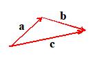
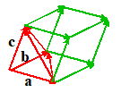
Let a and b be vectors. Then is also a vector. The vector c may be shown diagramatically by placing arrows representing a and b head to tail, as shown in the figure.
 Multiplication
1. Multiplication by a scalar. Let a be a
vector, and  a scalar. Then is a vector.
The direction of is parallel to and its magnitude is given by .
a scalar. Then is a vector.
The direction of is parallel to and its magnitude is given by .
Note that you can form a unit vector n
which is parallel to a by setting .
2. 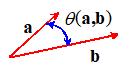 Dot Product (also called the scalar product). Let a and b be two vectors. The dot
product of a and b is a scalar denoted by ,
and is defined by
Dot Product (also called the scalar product). Let a and b be two vectors. The dot
product of a and b is a scalar denoted by ,
and is defined by
,
where
is the angle subtended by a and b. Note that ,
and . If and then if and only if ;
i.e. a and b are perpendicular.
3. 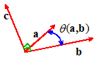 Cross
Product (also called the vector
product). Let a and b be two
vectors. The cross product of a and b is a vector denoted by . The
direction of c is perpendicular to a and b, and is chosen so that (a,b,c)
form a right handed triad, Fig. 3. The
magnitude of c is given by
Cross
Product (also called the vector
product). Let a and b be two
vectors. The cross product of a and b is a vector denoted by . The
direction of c is perpendicular to a and b, and is chosen so that (a,b,c)
form a right handed triad, Fig. 3. The
magnitude of c is given by
Note
that and .
Some useful vector identities
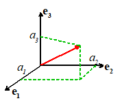
3.1.3 Cartesian components of vectors
Let
be three mutually perpendicular unit vectors
which form a right handed triad, Fig. 4.
Then are said to form and orthonormal basis. The
vectors satisfy
We
may express any vector a as a
suitable combination of the unit vectors ,
and . For example, we may write
where
 are scalars, called
the components of a in the basis . The components of a have a simple physical interpretation. For example, if we evaluate the dot product we find that
are scalars, called
the components of a in the basis . The components of a have a simple physical interpretation. For example, if we evaluate the dot product we find that
in view of the properties
of the three vectors ,
and . Recall that
Then, noting that ,
we have
Thus,
 represents the
projected length of the vector a in the direction of ,
as illustrated in the figure. Similarly,
and may be shown to represent the projection of in the directions and
represents the
projected length of the vector a in the direction of ,
as illustrated in the figure. Similarly,
and may be shown to represent the projection of in the directions and  , respectively.
The
advantage of representing vectors in a Cartesian basis is that vector addition
and multiplication can be expressed as simple operations on the components of
the vectors. For example, let a, b
and c be vectors, with components ,
and ,
respectively. Then, it is straightforward
to show that
3.1.4 Change of basis
Let
a be a vector, and let be a Cartesian basis. Suppose that the components of a in the basis are known to be . Now, suppose that we wish to compute the
components of a in a second
Cartesian basis, . This means we wish to find components ,
such that
To do so, note that
This transformation is
conveniently written as a matrix operation
,
where
is a matrix consisting of the components of a in the basis ,
is a matrix consisting of the components of a in the basis ,
and  is a `rotation matrix’
as follows
is a `rotation matrix’
as follows
Note
that the elements of have a simple physical
interpretation. For example, ,
where is the angle between the and  axes. Similarly where is the angle between the and
  axes. In practice, we usually know the angles
between the axes that make up the two bases, so it is simplest to assemble the
elements of by putting the cosines
of the known angles in the appropriate places.
axes. In practice, we usually know the angles
between the axes that make up the two bases, so it is simplest to assemble the
elements of by putting the cosines
of the known angles in the appropriate places.
Index notation provides
another convenient way to write this transformation:
You
don’t need to know index notation in detail to understand this all you need to know is that
The same approach may be
used to find an expression for in terms of . If you work through the details, you will
find that
Comparing this result with
the formula for in terms of ,
we see that
where
the superscript T denotes the
transpose (rows and columns interchanged). The transformation matrix is therefore orthogonal, and satisfies
where [I] is the identity matrix.
3.1.5 Useful vector operations

Calculating areas
The
area of a triangle bounded by vectors a,
b¸and b-a is
The
area of the parallelogram shown in the picture is 2A.
Calculating
angles
The angle between two vectors a and b is
Calculating
the normal to a surface.
If two vectors a and b can be found
which are known to lie in the surface, then the unit normal to the surface is
If the surface is specified by a
parametric equation of the form ,
where s and t are two parameters and
r is the position vector of a point
on the surface, then two vectors which lie in the plane may be computed from
Calculating
Volumes
The volume of the parallelopiped defined by three vectors a, b,
c is
The volume of the tetrahedron shown outlined in red is V/6.
3.2 Vector Fields and Vector Calculus
3.2.1. Scalar field.
Let be a Cartesian basis with origin O in three
dimensional space. Let
denote
the position vector of a point in space.
A scalar field is a scalar
valued function of position in space. A
scalar field is a function of the components of the position vector, and so may
be expressed as .
The value of  at a particular point
in space must be independent of the choice of basis vectors. A scalar field may be a function of time (and
possibly other parameters) as well as position in space.
at a particular point
in space must be independent of the choice of basis vectors. A scalar field may be a function of time (and
possibly other parameters) as well as position in space.
3.2.2. Vector field
Let be a Cartesian basis with origin O in three
dimensional space. Let
denote
the position vector of a point in space.
A vector field is a vector
valued function of position in space. A
vector field is a function of the components of the position vector, and so may
be expressed as . The vector may also be expressed as
components in the basis
The
magnitude and direction of  at a particular point
in space is independent of the choice of basis vectors. A vector field may be a function of time
(and possibly other parameters) as well as position in space.
at a particular point
in space is independent of the choice of basis vectors. A vector field may be a function of time
(and possibly other parameters) as well as position in space.
3.2.3. Change of basis for scalar fields.
Let
be a Cartesian basis with origin O in three
dimensional space. Express the position vector of a point relative to O in as
and let be a scalar field.
Let
be a second Cartesian basis, with origin
P. Let denote the position vector of P relative to O. Express the position vector
of a point relative to P in as
To
find ,
use the following procedure. First,
express p as components in the basis ,
using the procedure outlined in Section 1.4:
where
or, using index notation
where the transformation
matrix is defined in Sect 1.4.
Now, express c as components in ,
and note that
so that
3.2.4. Change of basis for vector fields.
Let
be a Cartesian basis with origin O in three
dimensional space. Express the position vector of a point relative to O in as
and let be a vector
field, with components
Let
be a second Cartesian basis, with origin
P. Let denote the position vector of P relative to O. Express the position vector of
a point relative to P in as
To
express the vector field as components in and as a function of the components of p, use the following procedure. First, express in terms of using the procedure outlined for scalar fields
in the preceding section
for
k=1,2,3. Now, find the components of v
in using the procedure outlined in Section
1.4. Using index notation, the result is
3.2.5. Time derivatives of vectors
Let
a(t) be a vector whose magnitude and
direction vary with time, t. Suppose that is a fixed basis, i.e. independent of
time. We may express a(t)
in terms of components in the basis as
 .
.
The time derivative of a is defined using the usual rules of
calculus
,
or in component form as
The
definition of the time derivative of a vector may be used to show the following
rules
3.2.6. Using a rotating basis
It
is often convenient to express position vectors as components in a basis which
rotates with time. To write equations of
motion one must evaluate time derivatives of rotating vectors.
Let be a basis which rotates with instantaneous
angular velocity . Then,
3.2.7. Gradient of a scalar field.
Let
be a scalar field in
three dimensional space. The gradient of
is a vector field
denoted by  or ,
and is defined so that
or ,
and is defined so that
for every position r in space and for every vector a.
Let  be a Cartesian basis
with origin O in three dimensional space.
Let
be a Cartesian basis
with origin O in three dimensional space.
Let
denote
the position vector of a point in space.
Express as a function of the
components of r . The gradient of in this basis is then
given by
3.2.8. Gradient of a vector field
Let v be a vector field in three dimensional space. The gradient of v is a tensor field denoted by or ,
and is defined so that
for every position r in space and for every vector a.
Let be a Cartesian basis with origin O in three
dimensional space. Let
denote
the position vector of a point in space.
Express v as a function of
the components of r, so that . The gradient of v
in this basis is then given by
Alternatively, in index
notation
3.2.9. Divergence of a vector field
Let
v be a vector field in three dimensional
space. The divergence of v is a scalar field denoted by or . Formally, it is defined as (the trace of a tensor is the sum of its
diagonal terms).
Let be a Cartesian basis
with origin O in three dimensional space.
Let
denote
the position vector of a point in space.
Express v as a function of
the components of r: .
The divergence of v is then
3.2.10. Curl of a vector field.
Let
v be a vector field in three
dimensional space. The curl of v is a vector field denoted by or . It is best defined in terms of its components
in a given basis, although its magnitude and direction are not dependent on the
choice of basis.
Let be a Cartesian basis with origin O in three
dimensional space. Let
denote
the position vector of a point in space.
Express v as a function of
the components of r .
The curl of v in this basis is then given by
Using index notation, this
may be expressed as
3.2.11 The Divergence Theorem.
 Let V be a
closed region in three dimensional space, bounded by an orientable surface S. Let n denote the unit vector
normal to S, taken so that n points out of V. Let u be a vector
field which is continuous and has continuous first partial derivatives in some
domain containing T. Then
Let V be a
closed region in three dimensional space, bounded by an orientable surface S. Let n denote the unit vector
normal to S, taken so that n points out of V. Let u be a vector
field which is continuous and has continuous first partial derivatives in some
domain containing T. Then
alternatively, expressed in
index notation
For
a proof of this extremely useful theorem consult e.g. Kreyzig, Advanced Engineering Mathematics, Wiley, New York, (1998).
3.3 MATRICES
3.3.1 Definition
An matrix is a set of numbers, arranged in m rows and n columns
A square
matrix has equal numbers of rows and columns
A diagonal
matrix is a square matrix with elements such that  for
for 
The identity
matrix is a diagonal matrix for which all diagonal
elements
A symmetric
matrix is a square matrix with elements such that
A skew
symmetric matrix is a square matrix with elements such that
3.3.2 Matrix operations
Addition Let and be two matrices of order with elements and . Then
Multiplication
by a scalar. Let be a matrix with elements ,
and let k be a scalar. Then
Multiplication by a matrix. Let be a matrix of order with elements ,
and let be a matrix of order with elements  . The product is defined only if n=p, and is an matrix such that
Note that
multiplication is distributive and associative, but not commutative, i.e.
The multiplication of a vector by a matrix is a particularly
important operation. Let b and c be two vectors with n components, which we think of as matrices.
Let be an matrix.
Thus
Now,
i.e.
Transpose.
Let be a matrix of order with elements . The transpose of is denoted . If is an matrix such that ,
then ,
i.e.
Note that
Determinant The determinant is defined only for a square
matrix. Let be a matrix with components . The determinant of is denoted by or and is given by
Now, let be an matrix.
Define the minors of as the determinant formed by omitting the ith row and jth column of . For example, the minors and for a matrix are computed as follows. Let
Then
Define the cofactors of as
Then, the
determinant of the matrix is computed as follows
The result is the same whichever row i is chosen for the expansion.
For the particular case of a matrix
The determinant may also be
evaluated by summing over rows, i.e.
and as
before the result is the same for each choice of column j. Finally, note that

Inversion. Let be an matrix.
The inverse of is denoted by  and is defined such
that
and is defined such
that

The inverse of exists if and only if . A matrix which has no inverse is said to be singular. The inverse of a matrix may be computed explicitly,
by forming the cofactor matrix with components as defined in the preceding section. Then
In practice, it is faster to compute the inverse of a matrix
using methods such as Gaussian elimination.
Note that
For a diagonal matrix, the inverse is
For a matrix, the inverse is
Eigenvalues and eigenvectors. Let be an matrix, with coefficients . Consider the vector equation
(1)
where x is a vector with n
components, and is a scalar (which may be complex). The n
nonzero vectors x and corresponding
scalars which satisfy this equation are the eigenvectors and eigenvalues of .
Formally, eighenvalues and eigenvectors may be computed as
follows. Rearrange the preceding
equation to
(2)
This has nontrivial solutions for x only if the determinant of
the matrix vanishes.
The equation
is
an nth order polynomial which may be
solved for . In general the polynomial will have n roots, which may be complex. The eigenvectors may then be computed using
equation (2). For example, a matrix
generally has two eigenvectors, which satisfy
Solve the
quadratic equation to see that
The two
corresponding eigenvectors may be computed from (2), which shows that
so that, multiplying out the first row of the matrix (you can
use the second row too, if you wish since we chose to make the
determinant of the matrix vanish, the two equations have the same solutions. In fact, if ,
you will need to do this, because the first equation will simply give 0=0 when
trying to solve for one of the eigenvectors)
which are
satisfied by any vector of the form
where p and q are arbitrary real numbers.
It is often convenient to normalize
eigenvectors so that they have unit `length’.
For this purpose, choose p and q so
that . (For vectors of dimension n, the generalized dot product is
defined such that )
One
may calculate explicit expressions for eigenvalues and eigenvectors for any
matrix up to order ,
but the results are so cumbersome that, except for the results, they are virtually useless. In practice, numerical values may be computed
using several iterative techniques.
Packages like Mathematica, Maple or Matlab make calculations like this
easy.
The
eigenvalues of a real symmetric matrix are always real, and its eigenvectors
are orthogonal, i.e. the ith and jth eigenvectors (with ) satisfy .
The eigenvalues of a skew
symmetric matrix are pure imaginary.
Spectral
and singular value decomposition.
Let be a real symmetric matrix. Denote the n (real) eigenvalues of by ,
and let be the corresponding normalized eigenvectors, such that . Then, for any arbitrary vector b,
Let be a diagonal matrix which contains the n
eigenvalues of as elements of the diagonal, and let be a matrix consisting of the n eigenvectors as columns, i.e.
Then
Note that this gives
another (generally quite useless) way to invert
where is easy to compute since is diagonal.
Square
root of a matrix. Let be a real symmetric matrix.
Denote the singular value decomposition of by as defined above. Suppose that denotes the square root of ,
defined so that
One way to
compute is through the singular value decomposition of
where
3.4 Brief Introduction to Tensors
3.4.1 Examples of Tensors
The
gradient of a vector field is a good example of a tensor. Visualize a vector field: at every point in
space, the field has a vector value . Let represent the gradient of u. By definition, G enables you to calculate the change
in u when you move from a point x in space to a nearby point at :
G is a second order tensor. From
this example, we see that when you multiply a vector by a tensor, the result is
another vector.
This
is a general property of all second order tensors. A
tensor is a linear mapping of a vector onto another vector. Two examples, together with the vectors they
operate on, are:
The stress tensor
where n is
a unit vector normal to a surface, is the stress tensor and t is the traction vector acting on the surface.
The deformation gradient tensor
where dx is an infinitesimal line element in
an undeformed solid, and dw is the vector representing the
deformed line element.
3.4.2 Matrix representation
of a tensor
To
evaluate and manipulate tensors, we express them as components in a basis, just as for vectors. We can use the displacement gradient to
illustrate how this is done. Let be a vector field, and let represent the gradient of u. Recall the definition of G
Now,
let be a Cartesian basis, and express both du
and dx as components. Then,
calculate the components of du in terms of dx using the usual rules
of calculus
We could represent this as a
matrix product
From
this we see that G can be
represented as a matrix.
The elements of the matrix are known as the components of G in the basis. All second order
tensors can be represented in this form.
For example, a general second order tensor S could be written as
You
have probably already seen the matrix representation of stress and strain
components in introductory courses.
Since
S can be represented as a matrix,
all operations that can be performed on a matrix can also be performed on S.
Examples include sums and products, the transpose, inverse, and
determinant. One can also compute
eigenvalues and eigenvectors for tensors, and thus define the log of a tensor,
the square root of a tensor, etc. These
tensor operations are summarized below.
Note
that the numbers ,
,
… depend on the basis ,
just as the components of a vector depend on the basis used to represent the
vector. However, just as the magnitude
and direction of a vector are independent of the basis, so the properties of a
tensor are independent of the basis.
That is to say, if S is a
tensor and u is a vector, then the
vector
has
the same magnitude and direction, irrespective of the basis used to represent u, v,
and S.
3.4.3 The difference between a matrix and a tensor
If
a tensor is a matrix, why is a matrix not the same thing as a tensor? Well, although you can multiply the three
components of a vector u by any matrix,
the
resulting three numbers may or may not represent the components of a
vector. If they are the components of a vector, then the matrix represents the
components of a tensor A, if not,
then the matrix is just an ordinary old matrix.
To check whether are the components of a vector, you need to
check how change due to a change of basis. That is to say, choose a new basis, calculate
the new components of u in this
basis, and calculate the new matrix in this basis (the new elements of the
matrix will depend on how the matrix was defined. The elements may or may not change if they don’t, then the matrix cannot be the
components of a tensor). Then, evaluate
the matrix product to find a new left hand side, say . If are related to by the same transformation that was used to
calculate the new components of u,
then are the components of a vector, and,
therefore, the matrix represents the components of a tensor.
3.4.4 Creating a tensor using a dyadic product of two
vectors.
Let a and b be two
vectors. The dyadic product of a and b is a second order tensor S denoted by
.
with the property
for
all vectors u. (Clearly, this maps u onto a vector parallel to a
with magnitude )
The components of in a basis are
Note
that not all tensors can be constructed using a dyadic product of only two
vectors (this is because always has to be parallel to a, and therefore the representation
cannot map a vector onto an arbitrary vector).
However, if a, b, and c are three independent vectors (i.e. no two of them are parallel)
then all tensors can be constructed as a sum of scalar multiples of the nine
possible dyadic products of these vectors.
3.4.5. Operations on Second Order Tensors
Tensor components.
Let
be a Cartesian basis,
and let S be a second order
tensor. The components of S in may be represented as
a matrix
where
The representation of a
tensor in terms of its components can also be expressed in dyadic form as
This representation is
particularly convenient when using polar coordinates, as described in Appendix
E.
Addition
Let S and T be two tensors. Then is also a tensor.
Denote
the Cartesian components of U, S and
T by matrices as defined above. The components of U are then related to the components of S and T by
Product
of a tensor and a vector
Let u be a vector and S a
second order tensor. Then
is a vector.
Let
and denote the components of vectors u and v in a Cartesian basis ,
and denote the Cartesian components of S
as described above. Then
The product
is also a vector. In component form
Observe that (unless S is symmetric).
Product
of two tensors
Let T and S be two second
order tensors. Then is
also a tensor.
Denote the components of U, S
and T by matrices.
Then,
Note that tensor products, like matrix products, are not
commutative; i.e.
Transpose
Let S be a tensor. The transpose
of S is denoted by and is defined so that
Denote the components of S by a 3x3 matrix. The components of are then
i.e. the rows and columns
of the matrix are switched.
Note that, if A and B are two tensors, then
Trace
Let
S be a tensor, and denote the
components of S by a matrix.
The trace of S is denoted by
tr(S) or trace(S), and can be computed by summing the diagonals of the matrix of
components
More formally, let be any Cartesian basis. Then
The
trace of a tensor is an example of an invariant
of the tensor you get the same value for trace(S) whatever basis you use to define the
matrix of components of S.
Contraction.
Inner Product: Let S and
T be two second order tensors. The inner product of S and T is a scalar,
denoted by . Represent S and T by their
components in a basis. Then
Observe that ,
and also that ,
where I is the identity tensor.
Outer product: Let
S and T be two second order tensors.
The outer product of S and T is a scalar, denoted by . Represent S and T by their
components in a basis. Then
Observe that
Determinant
The
determinant of a tensor is defined as the determinant of the matrix of its
components in a basis. For a second
order tensor
Note that if S and T are two tensors, then
Inverse
Let
S be a second order tensor. The inverse of S exists if and only if ,
and is defined by
where  denotes the
inverse of S and I is the identity tensor.
denotes the
inverse of S and I is the identity tensor.
The
inverse of a tensor may be computed by calculating the inverse of the matrix of
its components. The result cannot be
expressed in a compact form for a general three dimensional second order
tensor, and is best computed by methods such as Gaussian elimination.
Eigenvalues and Eigenvectors (Principal values and
direction)
Let S be a second order tensor.
The scalars and unit vectors m which satisfy
are
known as the eigenvalues and eigenvectors of S, or
the principal values and principal directions of S. Note that may be complex. For a second order tensor in three
dimensions, there are generally three values of and three unique unit vectors m which satisfy this equation. Occasionally, there may be only two or one
value of . If this is the case, there are infinitely
many possible vectors m that satisfy
the equation. The eigenvalues of a
tensor, and the components of the eigenvectors, may be computed by finding the
eigenvalues and eigenvectors of the matrix of components (see A.3.2)
The
eigenvalues of a symmetric tensor are always real. The eigenvalues of a skew tensor are always
pure imaginary or zero.
Change of Basis.
Let
S be a tensor, and let be a Cartesian
basis. Suppose that the components of S in the basis are known to be
Now, suppose that we wish
to compute the components of S in a second Cartesian basis, . Denote these components by
To do so, first compute the
components of the transformation matrix [Q]
(this is the same matrix
you would use to transform vector components from to ).
Then,
or, written out in full
To prove this result, let u and v be vectors satisfying
Denote the components of u and v in the two bases by and ,
respectively. Recall that the vector
components are related by
Now, we could express the
tensor-vector product in either basis
Substitute for from above into the second of these two
relations, we see that
Recall that
so multiplying both sides
by [Q] shows that
so, comparing with the
first of equation (1)
as stated.
Invariants
Invariants of a tensor are functions of the tensor components
which remain constant under a basis change.
That is to say, the invariant has the same value when computed in two
arbitrary bases and .
A symmetric second order tensor always
has three independent invariants.
Examples of invariants are
1. The three eigenvalues
2. The determinant
3. The trace
4. The inner and outer products
These are not all
independent for example any of 2-4 can be calculated in
terms of 1.
3.4.6
Identity tensor The identity tensor I is the tensor such that, for any tensor S or vector v
In any basis, the identity
tensor has components
Symmetric Tensor A symmetric tensor S has
the property
The components of a
symmetric tensor have the form
so that there are only six
independent components of the tensor, instead of nine.
Skew Tensor A skew tensor S has the property
The components of a skew
tensor have the form
Orthogonal Tensors An orthogonal tensor S has
the property
An orthogonal tensor must
have ;
a tensor with is known as a proper orthogonal tensor.
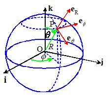
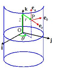
3.5 Vectors and Tensors in Spherical-Polar Coordinates
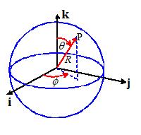
3.5.1 Specifying points in spherical-polar
coordinates
To
specify points in space using spherical-polar coordinates, we first choose two
convenient, mutually perpendicular reference directions (i and k in the
picture). For example, to specify
position on the Earth’s surface, we might choose k to point from the center of the earth towards the North Pole, and
choose i to point from the center of
the earth towards the intersection of the equator (which has zero degrees
latitude) and the Greenwich Meridian (which has zero degrees longitude, by
definition).
Then,
each point P in space is identified by three numbers, shown in the picture above. These
are not components of a vector.
In words:
R
is the distance of P from the origin
is the angle
between the k direction and OP
is the angle between the i direction and the projection of OP onto a plane through O normal
to k
By convention, we choose , and
3.5.2 Converting between Cartesian and
Spherical-Polar representations of points
When
we use a Cartesian basis, we identify points in space by specifying the
components of their position vector relative to the origin (x,y,z), such that When we use a spherical-polar coordinate
system, we locate points by specifying their spherical-polar coordinates
The formulas below relate
the two representations. They are
derived using basic trigonometry
3.5.3 Spherical-Polar representation of vectors
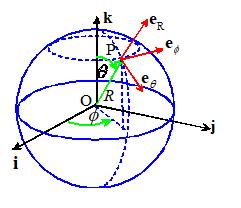 When we work with vectors in spherical-polar
coordinates, we abandon the {i,j,k}
basis. Instead, we specify vectors as
components in the basis shown in the figure. For example, an arbitrary vector a is written as ,
where denote the components of a.
When we work with vectors in spherical-polar
coordinates, we abandon the {i,j,k}
basis. Instead, we specify vectors as
components in the basis shown in the figure. For example, an arbitrary vector a is written as ,
where denote the components of a.
The basis is different for
each point P. In words
points along OP
is tangent to a line of constant longitude
through P
is tangent to a line of constant latitude
through P.
For
example if polar-coordinates are used to specify points on the Earth’s
surface, you can visualize the basis
vectors like this. Suppose you stand at
a point P on the Earths surface.
Relative to you: points vertically upwards; points due South; and points due East. Notice that the basis vectors
depend on where you are standing.
You
can also visualize the directions as follows.
To see the direction of ,
keep and fixed, and increase R. P is moving parallel to . To see the direction of ,
keep R and fixed, and increase .
P now moves parallel to . To see the direction of ,
keep R and fixed, and increase . P now moves parallel to . Mathematically, this concept can be expressed
as follows. Let r be the position vector of P.
Then
By
definition, the `natural basis’ for a coordinate system is the derivative of
the position vector with respect to the three scalar coordinates that are used
to characterize position in space (see Chapter 10 for a more detailed
discussion). The basis vectors for a
polar coordinate system are parallel to the natural basis vectors, but are
normalized to have unit length. In
addition, the natural basis for a polar coordinate system happens to be orthogonal.
Consequently, is an orthonormal basis (basis vectors have
unit length, are mutually perpendicular and form a right handed triad)
3.5.4 Converting vectors between Cartesian and
Spherical-Polar bases
Let be a vector, with components in the spherical-polar basis . Let denote the components of a in the basis {i,j,k}.
The two sets of components
are related by
while the inverse relationship
is
Observe
that the two 3x3 matrices involved in this transformation are transposes (and
inverses) of one another. The
transformation matrix is therefore orthogonal, satisfying ,
where denotes the 3x3 identity matrix.
Derivation: It is easiest to do the transformation by expressing
each basis vector as components in {i,j,k}, and then substituting.
To do this, recall that ,
recall also the conversion
and finally recall that by
definition
Hence, substituting for x,y,z and differentiating
Conveniently we find that .
Therefore
Similarly
while ,
so that
Finally, substituting
Collecting terms in i, j
and k, we see that
This is the result stated.
To show the inverse result,
start by noting that
(where we have used ).
Recall that
Substituting, we get
Proceeding in exactly the
same way for the other two components gives the remaining expressions
Re-writing the last three
equations in matrix form gives the result stated.
3.5.5
Spherical-Polar representation of tensors
The
triad of vectors is an orthonormal basis (i.e. the three basis
vectors have unit length, and are mutually perpendicular). Consequently, tensors can be represented as
components in this basis in exactly the same way as for a fixed Cartesian basis
. In particular, a general second order tensor S can be represented as a 3x3 matrix
You
can think of as being equivalent to ,
as ,
and so on. All tensor operations such as addition, multiplication by a vector,
tensor products, etc can be expressed in terms of the corresponding operations
on this matrix, as discussed in Section B2 of Appendix B.
The
component representation of a tensor can also be expressed in dyadic form as
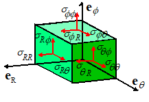 Furthermore, the physical significance of the components
can be interpreted in exactly the same way as for tensor components in a
Cartesian basis. For example, the
spherical-polar coordinate representation for the Cauchy stress tensor has the
form
Furthermore, the physical significance of the components
can be interpreted in exactly the same way as for tensor components in a
Cartesian basis. For example, the
spherical-polar coordinate representation for the Cauchy stress tensor has the
form
The component represents the traction component in direction
acting on an internal material plane with
normal ,
and so on. Of course, the Cauchy stress
tensor is symmetric, with
3.5.6 Constitutive equations in spherical-polar
coordinates
The
constitutive equations listed in Chapter 3 all relate some measure of stress in
the solid (expressed as a tensor) to some measure of local internal deformation
(deformation gradient, Eulerian strain, rate of deformation tensor, etc), also
expressed as a tensor. The constitutive
equations can be used without modification in spherical-polar coordinates, as
long as the matrices of Cartesian components of the various tensors are replaced
by their equivalent matrices in spherical-polar coordinates.
For
example, the stress-strain relations for an isotropic, linear elastic material
in spherical-polar coordinates read
HEALTH WARNING: If you are solving a problem involving anisotropic materials using
spherical-polar coordinates, it is important to remember that the orientation
of the basis vectors vary with position. For example, for an anisotropic, linear
elastic solid you could write the constitutive equation as
however,
the elastic constants would need to be represent the material
properties in the basis ,
and would therefore be functions of position (you would have to calculate them
using the lengthy basis change formulas listed in Section 3.2.11). In practice the results are so complicated
that there would be very little advantage in working with a spherical-polar
coordinate system in this situation.
3.5.7 Converting tensors between Cartesian and
Spherical-Polar bases
Let
S be a tensor, with components
in
the spherical-polar basis and the Cartesian basis {i,j,k}, respectively. The
two sets of components are related by
These
results follow immediately from the general basis change formulas for tensors
given in Appendix B.
3.5.8 Vector Calculus using Spherical-Polar
Coordinates
Calculating
derivatives of scalar, vector and tensor functions of position in
spherical-polar coordinates is complicated by the fact that the basis vectors
are functions of position. The results
can be expressed in a compact form by defining the gradient operator, which, in spherical-polar coordinates, has the
representation
In addition, the
derivatives of the basis vectors are
You can derive these
formulas by differentiating the expressions for the basis vectors in terms of {i,j,k}
and
evaluating the various derivatives. When differentiating, note that {i,j,k} are fixed, so their derivatives
are zero. The details are left as an
exercise.
The various derivatives of
scalars, vectors and tensors can be expressed using operator notation as
follows.
Gradient of a scalar function: Let denote a scalar function of position. The gradient of f is denoted by
Alternatively, in matrix
form
Gradient of a vector function Let be a vector function of position. The gradient
of v is a tensor, which can be
represented as a dyadic product of the vector with the gradient operator as
The
dyadic product can be expanded but when evaluating the derivatives it is
important to recall that the basis vectors are functions of the coordinates and consequently their derivatives do not
vanish. For example
Verify for yourself that
the matrix representing the components of the gradient of a vector is
Divergence of a vector function Let be a vector function of position. The
divergence of v is a scalar, which
can be represented as a dot product of the vector with the gradient operator as
Again,
when expanding the dot product, it is important to remember to differentiate
the basis vectors. Alternatively, the divergence can be expressed as ,
which immediately gives
Curl of a vector function Let be a vector function of position. The curl of v is a vector, which can be represented
as a cross product of the vector with the gradient operator as
The curl rarely appears in
solid mechanics so the components will not be expanded in full
Divergence of a tensor function. Let
be a tensor, with dyadic representation
The divergence of S is a vector, which can be represented
as
Evaluating
the components of the divergence is an extremely tedious operation, because
each of the basis vectors in the dyadic representation of S must be differentiated, in addition to the components
themselves. The final result (expressed
as a column vector) is
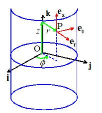
3.6 Vectors and Tensors in Cylindrical-Polar
Coordintes
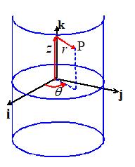
3.6.1 Specifying points in space using in
cylindrical-polar coordinates
To
specify the location of a point in cylindrical-polar coordinates, we choose an
origin at some point on the axis of the cylinder, select a unit vector k to be parallel to the axis of the
cylinder, and choose a convenient direction for the basis vector i, as shown in the picture. We then use the three numbers to locate a point inside the cylinder, as
shown in the picture. These are not components of a vector.
In words
r is the radial distance of P from the axis of the cylinder
is the angle between the i direction and the
projection of OP onto the i,j plane
z
is the length of the projection of OP on the axis of the cylinder.
By convention r>0 and
3.6.2 Converting between cylindrical polar and
rectangular cartesian coordinates
When
we use a Cartesian basis, we identify points in space by specifying the
components of their position vector relative to the origin (x,y,z), such that When we use a spherical-polar coordinate
system, we locate points by specifying their spherical-polar coordinates
The formulas below relate
the two representations. They are
derived using basic trigonometry
3.6.3 Cylindrical-polar representation of vectors
When
we work with vectors in spherical-polar coordinates, we specify vectors as
components in the .. basis shown in the figure.
For example, an arbitrary vector a
is written as ,
where denote the components of a.
The
basis vectors are selected as follows
is a unit vector normal to the cylinder at P
is a unit vector circumferential to the
cylinder at P, chosen to make a right handed triad
is parallel to the k vector.
You will see that the
position vector of point P would be expressed as
Note also that the basis
vectors are intentionally chosen to satisfy
The
basis vectors have unit length, are mutually perpendicular, and form a right
handed triad and therefore is an orthonormal basis. The basis vectors are parallel to (but not
equivalent to) the natural basis vectors for a cylindrical polar coordinate
system (see Chapter 10 for a more detailed discussion).
3.6.4 Converting vectors between Cylindrical and Cartesian
bases
Let
be a vector, with components in the spherical-polar basis . Let denote the components of a in the basis {i,j,k}.
The two sets of components
are related by
Observe
that the two 3x3 matrices involved in this transformation are transposes (and
inverses) of one another. The
transformation matrix is therefore orthogonal, satisfying ,
where denotes the 3x3 identity matrix.
The
derivation of these results follows the procedure outlined in E.1.4 exactly,
and is left as an exercise.
3.6.5 Cylindrical-Polar representation of tensors
The
triad of vectors is an orthonormal basis (i.e. the three basis
vectors have unit length, and are mutually perpendicular). Consequently, tensors can be represented as
components in this basis in exactly the same way as for a fixed Cartesian basis
. In particular, a general second order tensor S can be represented as a 3x3 matrix
You
can think of as being equivalent to ,
as ,
and so on. All tensor operations such as addition, multiplication by a vector,
tensor products, etc can be expressed in terms of the corresponding operations
on this matrix, as discussed in Section B2 of Appendix B.
The
component representation of a tensor can also be expressed in dyadic form as
3.6.6 Constitutive equations in cylindrical-polar
coordinates
The
constitutive equations listed in Chapter 3 all relate some measure of stress in
the solid (expressed as a tensor) to some measure of local internal deformation
(deformation gradient, Eulerian strain, rate of deformation tensor, etc), also
expressed as a tensor. The constitutive
equations can be used without modification in cylindrical-polar coordinates, as
long as the matrices of Cartesian components of the various tensors are
replaced by their equivalent matrices in spherical-polar coordinates.
For
example, the stress-strain relations for an isotropic, linear elastic material
in cylindrical-polar coordinates read
The
cautionary remarks regarding anisotropic materials in E.1.6 also applies to
cylindrical-polar coordinate systems.
3.6.7 Converting tensors between Cartesian and
Spherical-Polar bases
Let
S be a tensor, with components
in
the cylindrical-polar basis and the Cartesian basis {i,j,k}, respectively. The
two sets of components are related by
3.6.8 Vector Calculus using Cylindrical-Polar
Coordinates
Calculating
derivatives of scalar, vector and tensor functions of position in
cylindrical-polar coordinates is complicated by the fact that the basis vectors
are functions of position. The results
can be expressed in a compact form by defining the gradient operator, which, in spherical-polar coordinates, has the
representation
In addition, the nonzero
derivatives of the basis vectors are
The various derivatives of
scalars, vectors and tensors can be expressed using operator notation as
follows.
Gradient of a scalar function: Let denote a scalar function of position. The gradient of f is denoted by
Alternatively, in matrix
form
Gradient of a vector function Let be a vector function of position. The gradient
of v is a tensor, which can be
represented as a dyadic product of the vector with the gradient operator as
The
dyadic product can be expanded but when evaluating the derivatives it is
important to recall that the basis vectors are functions of the coordinate and consequently their derivatives may not
vanish. For example
Verify for yourself that
the matrix representing the components of the gradient of a vector is
Divergence of a vector function Let be a vector function of position. The
divergence of v is a scalar, which
can be represented as a dot product of the vector with the gradient operator as
Again,
when expanding the dot product, it is important to remember to differentiate
the basis vectors. Alternatively, the divergence can be expressed as ,
which immediately gives
Curl of a vector function Let be a vector function of position. The curl of v is a vector, which can be represented
as a cross product of the vector with the gradient operator as
The curl rarely appears in
solid mechanics so the components will not be expanded in full
Divergence of a tensor function. Let
be a tensor, with dyadic representation
The divergence of S is a vector, which can be represented
as
Evaluating
the components of the divergence is an extremely tedious operation, because
each of the basis vectors in the dyadic representation of S must be differentiated, in addition to the components
themselves. The final result (expressed
as a column vector) is
3.7 Index Notation for Vector and Tensor Operations
Operations
on Cartesian components of vectors and tensors may be expressed very
efficiently and clearly using index
notation.
3.7.1. Vector and tensor components.
Let
x be a (three dimensional) vector
and let S be a second order
tensor. Let be a Cartesian basis. Denote the components of
x in this basis by ,
and denote the components of S by
Using
index notation, we would express x
and S as
3.7.2.
Conventions and special symbols for index notation
Range
Convention: Lower case Latin subscripts (i, j, k…) have the range . The symbol denotes three components of a vector and . The symbol denotes nine components of a second order
tensor,
Summation
convention (Einstein convention): If an index is repeated in a product of
vectors or tensors, summation is implied over the repeated index. Thus
In
the last two equations, ,
and denote the component matrices of A, B and C.
The
Kronecker Delta: The symbol is known as the Kronecker delta, and has the
properties
thus
You can also think of as the components of the identity tensor, or a
identity matrix. Observe the following useful results
The
Permutation Symbol: The symbol has properties
thus
Note that
3.7.3. Rules of index
notation
1. The same index (subscript) may not
appear more than twice in a product of two (or more) vectors or tensors. Thus

are valid, but

are meaningless
2. Free indices on each term of an
equation must agree. Thus

are valid, but

are meaningless.
3. Free and
dummy indices may be changed without altering the meaning of an expression,
provided that rules 1 and 2 are not violated. Thus

3.7.4. Vector operations expressed using
index notation
Addition.
Dot
Product
Vector
Product
Dyadic
Product 
Change
of Basis. Let a be a vector. Let be a Cartesian basis,
and denote the components of a in
this basis by  . Let
. Let  be a second basis, and
denote the components of a in this
basis by . Then, define
be a second basis, and
denote the components of a in this
basis by . Then, define
where  denotes the angle
between the unit vectors
denotes the angle
between the unit vectors  and
and  . Then
3.7.5. Tensor
operations expressed using index notation.
Addition.
Transpose
Scalar
Products
Product
of a tensor and a vector
Product
of two tensors
Determinant
Change
of Basis. Let A be a second order tensor. Let be a Cartesian basis,
and denote the components of A in
this basis by . Let be a second basis, and denote the components
of A in this basis by  . Then, define

where denotes the angle
between the unit vectors and . Then

3.7.6. Calculus using index notation
The
derivative can be deduced by noting that and . Therefore
The
same argument can be used for higher order tensors
3.7.7. Examples of algebraic
manipulations using index notation
1.
Let a, b, c, d be vectors. Prove that
Express
the left hand side of the equation using index notation (check the rules for
cross products and dot products of vectors to see how this is done)
Recall
the identity
so
Multiply
out, and note that
(multiplying
by a Kronecker delta has the effect of switching indices…) so
Finally,
note that
and
similarly for other products with the same index, so that
2. The stressstrain relation
for linear elasticity may be expressed as
where and are the components of the stress and strain
tensor, and and denote Young’s modulus and Poisson’s
ratio. Find an expression for strain in
terms of stress.
Set i=j to see that
Recall that ,
and notice that we can replace the remaining ii by kk
Now, substitute for in the given stressstrain relation
3. Solve the equation
for
in terms of and
Multiply
both sides by  to see that
Substitute
back into the equation given for to see that
4. Let . Calculate
We
can just apply the usual chain and product rules of differentiation
5. Let . Calculate
Using
the product rule