Chapter 11

 

Analyzing solids with special shapes

 

 

Calculating the full 3D displacement field, along with all 9 stress and strain components in a solid can be difficult (even with the latest finite element software).  For some solids with special shapes, the analysis can be simplified by making assumptions about how the stress and strain vary in the solid.   This can be particularly helpful to analyze structural elements, such as rods, beams, plates and shells.

 

In this chapter we will discuss how to analyze deformation of straight beams and flat plates, to illustrate the main ideas.   There is a large literature on analysis of structural elements, which is often taught in a sequence of several courses, and cannot be discussed fully here.   Our main goal is to provide enough background in the subject so you can set up and interpret finite element simulations that include some of these structural elements

 

11.1 Analyzing Deformation and Motion of Straight Beams and Strings

 

We start by discussing simplified solid mechanics theories that describe motion of slender rods and beams.   The figure shows the problem to be solved.   To keep the discussion (reasonably) simple here, we will assume

 

 The solid is a straight beam, with a uniform cross-section (in FEA simulations, beams can be curved, and the cross-section can vary along the length of the beam)

 

 We will describe position and motion of the beam using a local Cartesian coordinate system with $e_3$ parallel to the axis of the beam.  In an ABAQUS simulation you may want to run an analysis with the beam pointing along some strange direction in space $–$ in this case it can be helpful to create a local coordinate system with the orientation shown when you create the part. 

 

 Deflections are small (FEA simulations can handle large deformations)

 

 We will neglect twisting of the cross section $–$ i.e. in the figure, the cross section does not rotate about the $e_3$ axis.   (You can include twist in FEA simulations; there are also several analytical methods for analyzing twisting of beams or rods, depending on the shape of the cross-section)

 

 

Characterizing the Geometry of the cross-section

 

In most FEA programs you can specify the geometry of the cross-section by simply entering relevant dimensions for standard cross-sections (circles, rectangles, I-beams, C and L sections and so on).  The software will compute all relevant integrated quantities internally.  

 

When we analyze deformation of straight elastic beams by hand, we start by introducing a convenient coordinate system: $e_3$ will be an axial unit vector, and  are two convenient directions in the plane of the cross-section (in FEA calculations the cross-sectional geometry is specified in a local coordinate system with $e_3$ tangent to the beam axis.   The orientation of the directions $e_1,e_2$ with respect to the global coordinate system must be specified separately).  We then calculate the following geometrical quantities:

1.      The cross-sectional area $A={\displaystyle \underset{A}{\int }dA}$ 

2.      The position of the neutral line in the cross section (this is a fiber in the beam that does not stretch as the beam bends)

$\overline{r}={\overline{x}}_1{e}_1+{\overline{x}}_2{e}_2=\frac{1}{A}{\displaystyle \underset{A}{\int }\left(x_1{e}_1+x_2{e}_2\right)dA}$

3.      The components of the area moment of inertia tensor for the cross-section

$\begin{array}{l}I=\left[\begin{array}{cc}{I}_{11}& -I_{12}\\ -I_{12}& I_{22}\end{array}\right]\\ I_{11}={\displaystyle \underset{A}{\int }{\left(x_2-{\overline{x}}_2^{}\right)}^{2}dA}{I}_{22}={\displaystyle \underset{A}{\int }{\left(x_1-{\overline{x}}_1^{}\right)}^{2}dA}{I}_{12}={\displaystyle \underset{A}{\int }\left(x_1-{\overline{x}}_1^{}\right)\left(x_2-{\overline{x}}_2^{}\right)dA}\end{array}$

 

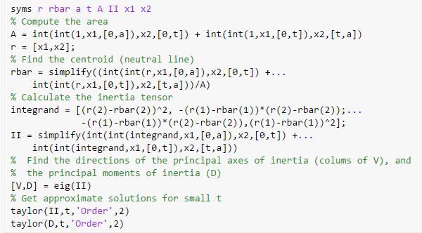
The integrals are always a pain to evaluate.   It is usually simplest to do them with a symbolic manipulation program.   As an example, here is a MATLAB live script that calculates the relevant quantities for a symmetric L-shaped cross-section.   To adapt this to different shapes you usually just need to work out how to handle the limits in the area integral $–$ the integrands don’t change.

 

The solution is

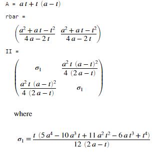
For small t/a we can use the approximation

Since I is a (2D) tensor, we can use all our secret tensor manipulation superpowers to manipulate it.   For example, the principal values and directions of I are useful (they are the eigenvalues and eigenvectors of I.   The eigenvectors can be visualized as a special basis in which I is diagonal; the corresponding eigenvalues are the values of $I_{11},I_{22}$ in this basis.  

For the L-shaped cross section Matlab says the principal axes of inertia (the eig command) are

The columns of V are the eigenvectors, but they are not unit vectors.  This tells us that

  $m_1=(-e_1+e_2)/\sqrt{2}{m}_2=(e_1+e_2)/\sqrt{2}$

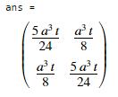
The principal moments of area are

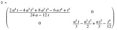
For small t/a this is

The top left diagonal is the moment of area about $m_1$ ; the bottom right is the moment of area about $m_2$.

 

The table below gives area moments of inertia for some simple shapes.   You can find more tabulated values online.

 

 

 

 

 

Approximating the deformation of a beam

 

The deformed shape of a straight beam is described by specifying the displacement $u(x_3)$ of each point on the neutral line of the cross-section, as a function of position along the length of the beam.  If the beam twists (not discussed here), it is also necessary to calculate the angle of rotation of the cross-section about the $e_3$ axis.  

 

Two additional geometric variables are used to describe the deformed geometry of a beam.  These are:

1.      The (small) rotation of the cross-section

${\theta }_1=-\frac{d{u}_2}{d{x}_3}{\theta }_2=\frac{d{u}_1}{d{x}_3}$

The sign conventions used to describe rotations is confusing $–$ the angles represent small rotations, in radians, about the $e_1,e_2$ axes.  The small rotation is a vector, and is related to the displacement by $\theta =e_3\times du/d{x}_3$. (If twist is included there is a third rotation angle that specifies the rotation of the cross section about the $e_3$ axis).

2.      The curvature of the beam

${\kappa }_1=\frac{d{\theta }_1}{d{x}_3}=-\frac{d^2{u}_2}{d{x}_3^2}{\kappa }_2=\frac{d{\theta }_2}{d{x}_3}=\frac{d^2{u}_1}{d{x}_3^2}$

The curvature is also a vector, and is related to the slope and displacement vectors by $\kappa =d\theta /d{x}_3=e_3\times d^{2}u/d{x}_3^2$ 

 

There are two main flavors of beam theory: the simplest one, called ‘Euler-Bernoulli’ beam theory, assumes that material fibers that are transverse to the neutral line remain transverse after deformation, as shown in the figure above (the solid blue lines are normal to the dashed blue line).  The axial strain distribution in the beam is then

${\epsilon }_{33}=-{\kappa }_2(x_1-{\overline{x}}_1)+{\kappa }_1(x_2-{\overline{x}}_2)$

 

The second version of beam theory (called ‘Timoshenko) beam theory allows material fibers transverse to the neutral line to rotate.   This theory is more complex (because you need to solve for the rotations of the transverse fibers) and won’t be discussed here, but it is available in most FEA packages.   Roughly, Timoshenko theory should be used for beams that are shorter than about 10 times their thickness; Euler-Bernoulli or Timoshenko theory can be used for long, slender beams (and will give the same predictions).

 

 

Describing external loads applied to beams

 

You can load a beam by

1.      Applying a distributed force (load per unit axial length) $p(x_3)$ along the length of the beam. 

2.      Either prescribing the transverse  displacement  $u(0),u(L)$ at the end, or applying forces P(0) P(L) at the ends of the beam (the forces can also be zero at a free end).  The forces are related to the tractions acting on the ends of the beam by

$P_i={\displaystyle \underset{A}{\int }{t}_{i}dA}$

3.      Either prescribing the rotation ${\theta }_1,{\theta }_2$ , or applying a moment $Q=Q_1{e}_1+Q_2{e}_2$ to the end of the beam (in more general theories a twist or twisting moment can also be applied parallel to the beam axis, but we have neglected twisting here to keep things simple). The components are related to the tractions acting on the end of the rod by

$Q_1={\displaystyle \underset{A}{\int }{x}_2{t}_{3}dA{Q}_2}=-{\displaystyle \underset{A}{\int }{x}_1{t}_{3}dA}$

 

 

 

 

 

 

 

 

 

 

Describing internal forces in beams

 

The forces in a beam are quantified by internal force and moment vectors acting on each cross-section.  To make this precise, introduce an imaginary cut perpendicular to the axis of the beam, as shown in the figure.  The stresses acting on an interior face with normal parallel to the $e_3$ direction exert resultant forces T, and bending moments M (if twisting is neglected $M_3=0$, but all three components have been shown to make it clear that M is a 3D vector).  

 

Beam theory calculates these resultant forces and moments directly (by solving the equations of motion or equilibrium in terms of T and M), instead of solving the 3D equations for the internal stresses.   Formally, the theory works by calculating the axial stress in the beam using the stress-strain relations and the strain-curvature relations, and then calculating the bending moments using

$M_1(x_3)={\displaystyle \underset{A}{\int }{\sigma }_{33}(x_2-{\overline{x}}_2)dA}{M}_2(x_3)=-{\displaystyle \underset{A}{\int }{\sigma }_{33}(x_1-{\overline{x}}_1)dA}$

The internal forces T in Euler-Bernoulli beam theory are constraint forces, which act to prevent the beam from stretching axially, and to keep transverse fibers perpendicular to the neutral line.  They can’t be calculated directly using the deformation and stress-strain laws, and instead are calculated using the momentum balance equations in the next section.

 

Note that T and M are vectors, and by default ABAQUS will report their components in the global coordinate system by default.

 

 

Moment-Curvature relations for elastic beams

 

In an elastic beam with Youngs modulus E, the bending moment vector is related to the curvature vector by

$M=EI\kappa \left[\begin{array}{c}{M}_1\\ M_2\end{array}\right]=E\left[\begin{array}{cc}{I}_{11}& -I_{12}\\ -I_{12}& I_{22}\end{array}\right]\left[\begin{array}{c}{\kappa }_1\\ {\kappa }_2\end{array}\right]$

 

It is easy to derive these:

1.      Recall that the axial strain in the beam is ${\epsilon }_{33}=-{\kappa }_2(x_1-{\overline{x}}_1)+{\kappa }_1(x_2-{\overline{x}}_2)$

2.      The elastic stress-strain law gives  ${\sigma }_{33}=-{\kappa }_2(x_1-{\overline{x}}_1)+{\kappa }_1(x_2-{\overline{x}}_2)$

3.      The bending moments are $M_1(x_3)={\displaystyle \underset{A}{\int }{\sigma }_{33}(x_2-{\overline{x}}_2)dA}{M}_2(x_3)=-{\displaystyle \underset{A}{\int }{\sigma }_{33}(x_1-{\overline{x}}_1)dA}$. 

4.      Finally, substitute for the stress and simplify using the definition of the inertia tensor

$\begin{array}{l}I=\left[\begin{array}{cc}{I}_{11}& -I_{12}\\ -I_{12}& I_{22}\end{array}\right]\\ I_{11}={\displaystyle \underset{A}{\int }{\left(x_2-{\overline{x}}_2^{}\right)}^{2}dA}{I}_{22}={\displaystyle \underset{A}{\int }{\left(x_1-{\overline{x}}_1^{}\right)}^{2}dA}{I}_{12}={\displaystyle \underset{A}{\int }\left(x_1-{\overline{x}}_1^{}\right)\left(x_2-{\overline{x}}_2^{}\right)dA}\end{array}$

 

 

 

 

 

Equations of motion for small deflections of straight beams subjected to significant axial force

 

Consider a beam with mass density $\rho$ , cross-sectional area A , which is subjected to a transverse distributed force per unit length $p=p_1{e}_1+p_2{e}_2+p_3{e}_3$, along with relevant forces or constraints at its ends.  The loading induces an acceleration vector $a=a_1{e}_1+a_2{e}_2$ and curvature vector $\kappa ={\kappa }_1{e}_1+{\kappa }_2{e}_2$ , along with internal forces $T=T_1{e}_1+T_2{e}_2+T_3{e}_3$ and bending moment. $M=M_1{e}_1+M_2{e}_2$ .  The equations of motion for the beam are

 

1. Linear momentum balance

$\frac{d{T}_1}{d{x}_3}+p_1\approx \rho A{a}_1\frac{d{T}_2}{d{x}_3}+p_2\approx \rho A{a}_2\frac{d{T}_3}{d{x}_3}+p_3\approx \rho A{a}_3$

2. Angular momentum balance

$\frac{d{M}_1}{d{x}_3}-T_2-{\theta }_1{T}_3\approx 0\frac{d{M}_2}{d{x}_3}+T_1-{\theta }_2{T}_3\approx 0$

 

These can also be written in more compact vector form

$\frac{dT}{d{x}_3}+p=\rho Aa\frac{dM}{d{x}_3}+e_3\times T-\theta T_3=0$

At the ends of the beam, the internal force T and M must satisfy boundary conditions

1.      Where forces are prescribed $T=-P{x}_3=0T=P{x}_3=L$

2.      Where moments are prescribed $M=-Q(x_3=0)M=Q(x_3=L)$

 

For an elastic beam, the transverse internal forces and curvature can all be eliminated to get two coupled differential equations for the transverse deflections of the beam

$\begin{array}{l}E\left(I_{22}\frac{d^4{u}_1}{d{x}_3^4}+I_{12}\frac{d^4{u}_2}{d{x}_3^4}\right)+\rho A\frac{d^2{u}_1}{d{t}^2}=\frac{d}{d{x}_3}\left(T_3\frac{d{u}_1}{d{x}_3}\right)+p_1\\ E\left(I_{12}\frac{d^4{u}_1}{d{x}_3^4}+I_{11}\frac{d^4{u}_2}{d{x}_3^4}\right)+\rho A\frac{d^2{u}_2}{d{t}^2}=\frac{d}{d{x}_3}\left(T_3\frac{d{u}_2}{d{x}_3}\right)+p_2\\ \frac{d{T}_3}{d{x}_3}+p_3\approx \rho A\frac{d^2{u}_3}{d{t}^2}\end{array}$

In terms of displacements, the possible boundary conditions are:

1.      Prescribed displacements $u(0)=u^{*}u(L)=u^{*}$ or

Prescribed forces $T=-P{x}_3=0T=P{x}_3=L$  where the two transverse forces are related to the displacements by

$\begin{array}{l}-E\left(I_{22}\frac{d^3{u}_1}{d{x}_3^3}+I_{12}\frac{d^3{u}_2}{d{x}_3^3}\right)+\frac{d{u}_1}{d{x}_3^{}}{T}_3=T_1\\ -E\left(I_{12}\frac{d^3{u}_1}{d{x}_3^4}+I_{11}\frac{d^3{u}_2}{d{x}_3^4}\right)+\frac{d{u}_2}{d{x}_3^{}}{T}_3=T_2\end{array}$

2.      Prescribed rotations $d{u}_1/d{x}_3={\theta }_2^{*}-d{u}_2/d{x}_3={\theta }_1^{*}$ or

Prescribed moments $M=-Q(x_3=0)M=Q(x_3=L)$ where the moment is related to the displacement by

$M_1=-E\left(I_{11}\frac{d^2{u}_2}{d{x}_3^2}+I_{12}\frac{d^2{u}_1}{d{x}_3^2}\right)M_2=E\left(I_{12}\frac{d^2{u}_2}{d{x}_3^2}+I_{22}\frac{d^2{u}_1}{d{x}_3^2}\right)$

 

Special cases:

 

Two limiting cases of these equations are often used.  

 

1.      Stretched string: If the bending resistance is small compared with the axial force ( $EI/(L^2{T}_3)<<1$ ) we get the equation of motion for a stretched string

$\begin{array}{l}\frac{d}{d{x}_3}\left(T_3\frac{d{u}_1}{d{x}_3}\right)+p_1=\rho A\frac{d^2{u}_1}{d{t}^2}\\ \frac{d}{d{x}_3}\left(T_3\frac{d{u}_2}{d{x}_3}\right)+p_2=\rho A\frac{d^2{u}_2}{d{t}^2}\\ \frac{d{T}_3}{d{x}_3}+p_3\approx \rho A\frac{d^2{u}_3}{d{t}^2}\end{array}$

In this case the equations for motion in the two transverse directions always decouple.  The boundary conditions at the ends of the string are:

(a)    Either: prescribed transverse displacement $u_1=u_1^{*},u_2=u_2^{*}$ or

prescribed transverse force

(b)   The axial force must satisfy $T_3=P_3(L)x_3=L{T}_3=-P_3(0)x_3=0$ 

Only displacements and forces can be prescribed at the ends of a string; the moments are always zero

 

2.      Beam with zero axial force.  In many cases the axial forces in the beam can be neglected.   In this case the equations of motion simplify to

$\begin{array}{l}E\left(I_{22}\frac{d^4{u}_1}{d{x}_3^4}+I_{12}\frac{d^4{u}_2}{d{x}_3^4}\right)+\rho A\frac{d^2{u}_1}{d{t}^2}=p_1\\ E\left(I_{12}\frac{d^4{u}_1}{d{x}_3^4}+I_{11}\frac{d^4{u}_2}{d{x}_3^4}\right)+\rho A\frac{d^2{u}_2}{d{t}^2}=p_2\end{array}$

It is often convenient to choose the $e_1,e_2$ directions so that $I_{12}=0$ .   The equations for the two transverse deflections then decouple.  

 

We close this section with two remarks:

1.      It is important to remember that these are approximate equations, and only apply to straight beams with small transverse deflections and no twist.  More general equations do exist, of course. 

2.      The linear momentum balance equations given here are in terms of force components in the fixed $\{e_1,e_2,e_3\}$ basis.  The same equations can be expressed in terms of components of internal and moment in a basis which rotates with the beam. These results look slightly different, but give the same governing equations for the displacement components. 

 

 

 

Example 1: The figure shows a flexible string (i.e. a beam with $EI/(L^2{T}_3)<<1$ ) subjected to a uniform transverse load p.    Calculate the transverse deflection.

 

Start by calculating the tension in the string.  The equation for axial force is

$\frac{d{T}_3}{d{x}_3}+p_3\approx \rho A{a}_3$

Since there is no axial force or acceleration, the tension is constant.   The boundary conditions at the end show $T_3=T_0$ .

 

We can now use the equation for transverse motion (we only need to worry about the vertical component, and there is no acceleration) which can be simplified to

$T_3\frac{d^2{u}_1}{d{x}_3^2}+p_1=0$

We don’t even need Matlab to solve this:

$u_1=-\frac{p_1{x}_3^2}{2T_3}+A{x}_3+B$

The transverse deflection is zero at $x_3=0,x_3=L$ , which shows that $B=0,A=p_1/(2L{T}_3)$ .  The solution is therefore

$u_1=\frac{p_1}{2T_3}{x}_3(L-x_3)$

 

 

Example 2:  The figure shows a cantilever beam with an L-shaped cross-section.  Its moment of inertia tensor can be approximate by

$I=\frac{a^{3}t}{8}\left[\begin{array}{cc}5/3& 1\\ 1& 5/3\end{array}\right]$

The beam is prevented from displacing or rotating at $x_3=0$ and is subjected to a vertical force P at $x_3=L$ .   Calculate the deflections $u_1,u_2$ 

 

For a beam in static equilibrium, with no axial load, and with no loads applied along the length of the beam we have that

 

$E\left(I_{22}\frac{d^4{u}_1}{d{x}_3^4}+I_{12}\frac{d^4{u}_2}{d{x}_3^4}\right)=0E\left(I_{12}\frac{d^4{u}_1}{d{x}_3^4}+I_{11}\frac{d^4{u}_2}{d{x}_3^4}\right)=0$

 

The boundary conditions are

1.      Zero displacement and rotation at $x_3=0$$u_1=u_2=d{u}_1/d{x}_3=d{u}_2/d{x}_3=0$ 

2.      Zero moment at $x_3=L$

$-E\left(I_{11}\frac{d^2{u}_2}{d{x}_3^2}+I_{12}\frac{d^2{u}_1}{d{x}_3^2}\right)=0E\left(I_{12}\frac{d^2{u}_2}{d{x}_3^2}+I_{22}\frac{d^2{u}_1}{d{x}_3^2}\right)=0$

3.      Prescribed force at $x_3=L$

$\begin{array}{l}-E\left(I_{22}\frac{d^3{u}_1}{d{x}_3^3}+I_{12}\frac{d^3{u}_2}{d{x}_3^3}\right)=0\\ -E\left(I_{12}\frac{d^3{u}_1}{d{x}_3^3}+I_{11}\frac{d^3{u}_2}{d{x}_3^3}\right)=P\end{array}$

It is not hard to solve these by hand $–$ the general solution for $u_1,u_2$ are just polynomials with unknown coefficients $–$ but it’s terribly boring to do the algebra.   A MATLAB ‘Live script’ is much faster

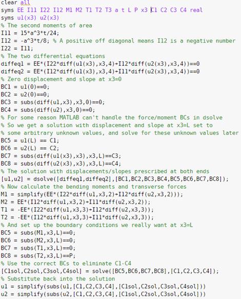
The MATLAB solution is shown.

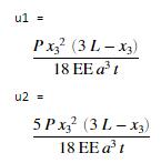
Notice that a vertical load causes a horizontal, as well as vertical displacement.   This is because the cross-section is unsymmetric $–$ if the beam deflected only vertically, the vertical side of the L would be in compression near its top, which would exert a non-zero moment on the cross-section about the $e_2$ axis.

 

 

 

Analyzing beams in ABAQUS

 

We end this section by discussing briefly how to set up an ABAQUS simulation that contains beams.

 

Part module:

1.      To create a beam in the ‘Part’ module, use Part->Create New and then select a 3D deformable object with a ‘Wire’ base feature.   Then draw a line that will define the shape of the beam.

2.      If you create a curved beam, you might find it helpful to create one or more local coordinate systems with axes oriented tangent and perpendicular to the beam.  It is usually easiest to make the x direction of the new system tangent to the beam.   You can do this by selecting Tools > Datum… and clicking the CSYS box.  There are a few different options for creating local coordinate systems.  If you select the ‘3 points’ method, ABAQUS will ask you to select an origin for your coordinate system, and then will ask you to put in coordinates (in the global coordinate system) for an origin, a point that lies on the x axis of the new system, and a second point in the new system that should lie in the current global x-y plane (this is confusing $–$ just try it a few times to figure out what it does). 

 

Property module

 

In the ‘Property’ module you will need to define the properties of the beam cross section. 

1.      Define a set of material properties in the usual way (Material, Create New, etc).  

2.      Then create a profile (Profile, Create new); select the shape and then enter the relevant geometric variables. 

3.      Next, create a beam section by going to Section > Create… and select Beam.  You can then select the profile and material you want to use to define your beam section.   The ‘Section integration’ will calculate the moment of inertia tensor for an elastic beam, or for other materials will integrate the stresses on the fly to calculate moments and shear forces.   Selecting ‘During analysis’ is the safest option.

4.      Once the section is created, you can assign it to the relevant section of the beam (Assign > Section).

5.      Finally you need to specify the orientation of the cross section of the beam.   Select Assign > Beam section orientation, then enter the information requested.  The default option makes the ‘1’ direction of the profile parallel to the z global coordinate direction.

 

Assembly module: There is nothing special about the assembly modules for beams. 

 

 

Interaction module

 You often need to analyze a structure consisting of a number of separate beams connected together.  You will need to create each beam as a separate part, and then specify how they are connected in the interaction module.   To do this,

1.      Select Constraint> Create

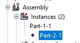
2.      Select ‘Node Region’ from the menu and then select the end of one of the two beams you want to connect.   Accept the choice (if it is the correct one!) then select the end of the second beam.  If you need to, you can hide members in the assembly by going to the Assembly tab in the model database tree, expand the ‘Instances’ branch, and then right click the part you want to hide.   Annoyingly if you do this at the wrong time it will end the constraint creation.   Usually if you select the first beam with all the parts shown (this will select the beam that was added to the assembly last), then wait until the ‘node region’ button appears for the second beam, you can operate the ‘hide’ and ‘show’ buttons without leaving the constraint definition menu..  

3.      In the constraint menu you can choose whether you want to connect the beams with a welded joint (check the Tie rotational DOF box) or a pin joint (uncheck the tie rotational DOF box).

 

 

Step module

 

You can define a ‘step’ in the usual way.  To get the simple small deflection version of beam theory defined in these notes, make sure the NLGEOM option is not selected.    If you select NLGEOM, ABAQUS will do a large displacement/rotation calculation.   These can be highly nonlinear and if you run a simulation without thinking through the proper magnitudes for loads and section properties, the analysis is likely to fail.

 

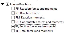
If you want ABAQUS to display the internal forces and moments in your beam, you will need to request that they be stored during the analysis.  To do this, select Output > Field Output Requests > Create and make sure the ‘Section Forces and Moments’ box is checked in the ‘Forces/Reactions’ list

 

 

Load Module

 

For the most part, you can define boundary conditions and forces in the Load module in the same way that you would for a 3D solid part.   The differences are:

1.      In beam analysis, the nodes have rotational as well as translational degrees of freedom (because you need to be able to specify slopes/moments acting on the beam).   The rotational degrees of freedom are shown as UR1, UR2, UR3 in the ‘Boundary condition’ definition window.   For small rotations, the three components of the rotation vector $\theta$ defined in these notes (in radians) $–$ you can select what coordinate system you want to use to define its components.    Large rotation don’t behave like vectors -  in this case ABAQUS uses UR1, UR2, UR3 to be the components in the axis-angle description of the rotation tensor.  The direction is the axis of rotation, and the magnitude is the rotation angle about the axis.

2.      You can apply moments to beams. 

 

 

 

 

Mesh Module

 

You will need to mesh your beams $–$ to do this, ‘seed’ them with nodes in the usual way, then mesh the part (or instance, whichever ABAQUS lets you do).   The default element types usually work; but as always with mesh design it is sensible to run the analysis with several different element types and meshes to check mesh sensitivity.   If the choice of element type or mesh makes a difference, you will need to decide which element type and mesh gives the most accurate solution.

 

Job Module $–$ set up jobs in the usual way.

 

Visualization Module

 

You can display displacements in the usual way.

 

ABAQUS will also display section forces and moments, and will also plot stresses in your beam.  Interpreting what is shown is tricky.

 

1.   To display internal forces in the beam (the vector T defined in these notes) select Result > Field Output and the select  from the menu.  The sign convention is confusing: SF1 is the axial force in the beam, SF2 and SF3 are the forces in the local (1) and (2) coordinate system for the beam (you defined these in the Property module).   

2.   To display internal moments select .  The variables SM1, SM2 are the bending moments about the local ‘1’ and ‘2’ axes, and SM3 is the twisting moment.

3.   ABAQUS also allows you to display stresses in the beam.   Since the stress varies with position in the cross-section you need to select which point in the cross-section to use: you can select the points using the Section Points… button in the Field Output selection window.

 

 

 

11.2 Analyzing Deformation and Motion of Flat Plates

 

We next consider simplified solid mechanics theories that describe motion of flat plates.   The figure shows the problem to be solved.   To keep the discussion (reasonably) simple here, we will assume

 

 The solid is a flat plate, with a uniform thickness h (in FEA simulations, plates can be curved (then they are called shells), and the thickness can vary)

 

 We will describe position and motion of the beam using a local Cartesian coordinate system with $e_3$ perpendicular to the plate.  In an ABAQUS simulation you may want to run an analysis with the beam pointing along some strange direction in space $–$ in this case it can be helpful to create a local coordinate system with the orientation shown when you create the part. 

 

 Deflections are small (FEA simulations can handle large deformations)

 

 

Approximating the deformation of a plate

 

The deformed shape of a flat plate is described by specifying the displacement $u(x_1,x_2)$ of each point on the centerline of the a function of position in the plane. 

 

Two additional geometric variables are used to describe the deformed geometry of a beam.  These are:

3.      The (small) rotation of the cross-section

${\theta }_1=\frac{d{u}_3}{d{x}_2}{\theta }_2=-\frac{d{u}_3}{d{x}_1}$

The angles represent small rotations, in radians, about the $e_1,e_2$ axes.  The small rotation is a vector, and is related to the displacement by $\theta =-e_3\times \nabla u$.

4.      The curvature of the plate

${\kappa }_{11}=\frac{d{\theta }_2}{d{x}_1}=-\frac{{\partial }^2{u}_3}{\partial x_1^2}{\kappa }_{12}={\kappa }_{21}=\frac{d{\theta }_2}{d{x}_1}=\frac{d{\theta }_1}{d{x}_2}=-\frac{{\partial }^2{u}_3}{\partial x_1\partial x_2}{\kappa }_{22}=-\frac{d{\theta }_1}{d{x}_2}=-\frac{{\partial }^2{u}_3}{\partial x_2^2}$

The curvature is a (2D) tensor, and is related to the rotation vector by $\kappa =\nabla \theta$ 

 

There are two main flavors of plate: the simplest one, called ‘Kirchhoff’ theory, assumes that material fibers that are transverse to the plane of the plate remain transverse after deformation, as shown in the figure above (the solid blue lines are normal to the dashed blue line).  The strain distribution in the plate is then

${\epsilon }_{11}=\frac{\partial u_1}{\partial x_1}+x_3{\kappa }_{11}{\epsilon }_{12}=\frac{1}{2}\left(\frac{\partial u_1}{\partial x_2}+\frac{\partial u_2}{\partial x_1}\right)+x_3{\kappa }_{12}{\epsilon }_{22}=\frac{\partial u_2}{\partial x_2}+x_3{\kappa }_{22}$

 

The second version of beam theory (called ‘Reissner-Mindlin’ beam theory) allows material fibers transverse to the neutral line to rotate.   This theory is more complex (because you need to solve for the rotations of the transverse fibers) and won’t be discussed here, but it is available in most FEA packages.   Roughly, Kirchoff theory should be used for plates that have width less than than about 10 times their thickness; Kirchoff or Reissner theory can be used for wide, thin plates (and will give the same predictions).

 

 

Describing external loads applied to plates

 

To keep things simple, we consider two types of external loading:

1.      A transverse pressure $p(x_1,x_2)$ acting normal to the surface of the plate, and

2.      A uniform force per unit length P acting normal to the perimeter of the plate.

In more general treatments, it is possible to apply forces acting transverse to the edge of the plate, as well as moments that cause the edge of the plate to rotate.   It is also possible to make P vary around the perimeter.

 

 

 

 

Internal forces in plates

 

The forces in a plate are quantified by internal force and moment tensors acting on each cross-section.  To make this precise, cut a square element from the plate with planes normal to the coordinate axes as shown in the figure.  A set of resultant forces and moments act on the exposed faces:

 

 The moments $M_{ij}$ are defined by

$M_{11}={\displaystyle \underset{-h/2}{\overset{h/2}{\int }}{\sigma }_{11}{x}_{3}d{x}_3}{M}_{12}=M_{21}={\displaystyle \underset{-h/2}{\overset{h/2}{\int }}{\sigma }_{12}{x}_{3}d{x}_3}{M}_{22}={\displaystyle \underset{-h/2}{\overset{h/2}{\int }}{\sigma }_{22}{x}_{3}d{x}_3}$ 

The physical significance of the components $M_{ij}$ is illustrated in the figure: $M_{1j}$ characterizes the moment per unit length acting on planes inside the shell that are normal to the $e_1$ direction, while $M_{2j}$ characterizes the moment per unit length acting on planes that are normal to $e_2$.  Note that $M_{i1}$ represents a moment about the $e_2$ axis, while $M_{i2}$ is a moment acting about the $-e_1$ axis. This can be expressed mathematically as $M=M_{\alpha \beta }{e}_{\alpha }\otimes (m_3\times e_{\beta })$ where the repeated indices $\alpha ,\beta$ are summed over 1 and 2, but this expression is only helpful if you are really good at visualizing dyadic and cross products.

 

 The in-plane forces $T_{ij}$ are defined by

$T_{11}={\displaystyle \underset{-h/2}{\overset{h/2}{\int }}{\sigma }_{11}d{x}_3}{T}_{12}=T_{21}={\displaystyle \underset{-h/2}{\overset{h/2}{\int }}{\sigma }_{12}d{x}_3}{T}_{22}={\displaystyle \underset{-h/2}{\overset{h/2}{\int }}{\sigma }_{22}d{x}_3}$

They represent resultant forces exerted by stresses on the internal planes: $T_{1j}$ are the components of force acting on the plane perpendicular to the $e_1$ direction, while $T_{2j}$ are those acting on the plane perpendicular to the $e_2$ direction.  In general, all three components of resultant force can be different.  But here, we consider only the simple case of uniform transverse loading applied to the perimeter of the plate.  Under these conditions the internal forces satisfy $T_{11}=T_{22}=T_0{T}_{12}=0$ , where $T_0$ is the magnitude of the transverse force.

  

 The transverse forces $V_1,V_2$ represent forces acting in the $e_3$ direction on planes perpendicular to the $e_1$ and $e_2$ direction, respectively.

 

 

Moment-Curvature and force-strain relations for elastic plates

 

The internal forces are related to the curvatures and strains by

$\left[\begin{array}{c}{T}_{11}\\ T_{22}\\ T_{12}\end{array}\right]=\frac{Eh}{(1-{\nu }^2)}\left[\begin{array}{ccc}1& \nu & 0\\ \nu & 1& 0\\ 0& 0& (1-\nu )\end{array}\right]\left[\begin{array}{c}\partial u_1/\partial x_1\\ \partial u_2/\partial x_2\\ (\partial u_1/\partial x_2+\partial u_2/\partial x_1)/2\end{array}\right]\left[\begin{array}{c}{M}_{11}\\ M_{22}\\ M_{12}\end{array}\right]=\frac{E{h}^3}{12(1-{\nu }^2)}\left[\begin{array}{ccc}1& \nu & 0\\ \nu & 1& 0\\ 0& 0& (1-\nu )\end{array}\right]\left[\begin{array}{c}{\kappa }_{11}\\ {\kappa }_{22}\\ {\kappa }_{12}\end{array}\right]$

 

It is easy to derive these: the plate is in a state of plane stress: the stresses are therefore related to the strains by

$\left[\begin{array}{c}{\sigma }_{11}\\ {\sigma }_{22}\\ {\sigma }_{12}\end{array}\right]=\frac{E}{(1-{\nu }^2)}\left[\begin{array}{ccc}1& \nu & 0\\ \nu & 1& 0\\ 0& 0& (1-\nu )\end{array}\right]\left[\begin{array}{c}{\epsilon }_{11}\\ {\epsilon }_{22}\\ {\epsilon }_{12}\end{array}\right]$

Substituting for the strains in terms of displacements and curvatures, and evaluating the integrals, gives the results stated.

 

The transverse forces $V_1,V_2$ cannot be determined directly from the curvatures or motion of the plate.  They represent constraint forces, which act to ensure that lines perpendicular to the mid-plane of the plate remain perpendicular after the plate deforms.   They can be calculated from the linear and angular momentum balance equations given in the next section.

 

 

Equations of motion for small deflections of flat plates subjected to significant in-plane force

 

Consider a plate with mass density $\rho$ , thickness h , which is subjected to a transverse distributed force per unit area $p=p_3{e}_3$, along with relevant forces or constraints at its edges.  The loading induces a transverse displacement $u_3$  acceleration vector $a=a_3{e}_3$ and curvature tensor components ${\kappa }_{11},{\kappa }_{12},{\kappa }_{22}$  , along with internal forces $T_{11}=T_{22}=T_0,T_{12}=0$ and bending moments $M_{11},M_{22},M_{12}$ .  The equations of motion for the plate are

 

1.      Linear momentum: (transverse motion)

$\frac{\partial V_1}{\partial x_1}+\frac{\partial V_2}{\partial x_2}+p_3=\rho h\frac{{\partial }^2{u}_3}{d{t}^2}$

2.      Angular momentum

    $\frac{\partial M_{11}}{\partial x_1}+\frac{\partial M_{12}}{\partial x_2}-T_0{\theta }_2-V_1\approx 0\frac{\partial M_{21}}{\partial x_1}+\frac{\partial M_{22}}{\partial x_2}+T_0{\theta }_1-V_2\approx 0$

 

 

These equations can be combined to eliminate V

$\frac{{\partial }^2{M}_{11}}{\partial x_1^2}+2\frac{{\partial }^2{M}_{12}}{\partial x_1\partial x_2}+\frac{{\partial }^2{M}_{22}}{\partial x_2^2}-T_0({\kappa }_{11}+{\kappa }_{22})+p_3=\rho h\frac{{\partial }^2{u}_3}{d{t}^2}$

This result can also be expressed in terms of displacement as

$\frac{E{h}^3}{12(1-{\nu }^2)}\left(\frac{{\partial }^4{u}_3}{\partial x_1^4}+2\frac{{\partial }^4{u}_3}{\partial x_1^2\partial x_2^2}+\frac{{\partial }^4{u}_3}{\partial x_2^4}\right)-T_0\left(\frac{{\partial }^2{u}_3}{\partial x_1^2}+\frac{{\partial }^2{u}_3}{\partial x_2^2}\right)+\rho h\frac{{\partial }^2{u}_3}{d{t}^2}=p_3$

 

The equation can also be written in polar coordinates as

$\frac{E{h}^3}{12(1-{\nu }^2)}{\left(\frac{{\partial }^2}{\partial r^2}+\frac{1}{r}\frac{\partial }{\partial r}+\frac{1}{r^2}\frac{{\partial }^2}{\partial {\theta }^2}\right)}^2{u}_3-T_0\left(\frac{{\partial }^2}{\partial r^2}+\frac{1}{r}\frac{\partial }{\partial r}+\frac{1}{r^2}\frac{{\partial }^2}{\partial {\theta }^2}\right)u_3+\rho h\frac{{\partial }^2{u}_3}{d{t}^2}=p_3$

 

 

Edge boundary conditions.  The edge of the plate is characterized by a curve C that lies in the mid-plane of the shell, encircling $e_3$ in a counterclockwise sense.   We let $s$ denote arc-length measured around C from some convenient origin, and use $\tau ={\tau }_{\alpha }{e}_{\alpha }$ and $n=e_3\times \tau$ denote unit vectors tangent and normal to C.  Elementary plate theory offers the following choices of boundary condition for each point on C:

1. Part of the boundary of the plate $C_1$ may be clamped, i.e. rotations and displacement of the boundary are completely prevented. The transverse displacement must then satisfy

$u_3=n_1\frac{\partial u_3}{\partial x_1}+n_2\frac{\partial u_3}{\partial x_2}=0$ on $C_1$.

2. Part of the boundary $C_2$ may be simply supported, i.e. the boundary of the plate is prevented from moving, but is permitted to rotate freely about the tangent vector $\tau$.  In this case the transverse displacement and internal moment must satisfy

$u_3=0M_{11}{n}_1^2+2M_{12}{n}_1{n}_2+M_{22}{n}_2^2=0$

3. Part of the boundary $C_3$ may be free, i.e. the boundary is free to both translate and rotate.  In this case the transverse shear force and internal moment must satisfy

$n_1{V}_1+n_2{V}_2+\frac{\partial }{\partial s}\left[M_{11}{n}_1{\tau }_1+2M_{12}{n}_1{\tau }_2+M_{22}{n}_2{\tau }_2\right]=0M_{11}{n}_1^2+2M_{12}{n}_1{n}_2+M_{22}{n}_2^2=0$

 

 

Special Cases

 

There are two special cases of these equations

1.      Stretched Membrane If the bending resistance is small compared with the in plane tension $E{h}^3/L^2{T}_0<<1$ we get the equation of motion for a biaxially stretched membrane

$T_0\left(\frac{{\partial }^2{u}_3}{\partial x_1^2}+\frac{{\partial }^2{u}_3}{\partial x_2^2}\right)+p_3=\rho h\frac{{\partial }^2{u}_3}{d{t}^2}$

or in polar coordinates

$T_0\left(\frac{{\partial }^2}{\partial r^2}+\frac{1}{r}\frac{\partial }{\partial r}+\frac{1}{r^2}\frac{{\partial }^2}{\partial {\theta }^2}\right)u_3+p_3=\rho h\frac{{\partial }^2{u}_3}{d{t}^2}$

The possible boundary conditions for a biaxially stretched membrane are:

(a)    Either prescribed transverse displacements at the edge of the membrane  $u_3=u^{*}$ or

Prescribed transverse force at the membrane edge $T_0(n_{1}d{u}_3/d{x}_1+n_{2}d{u}_3/d{x}_2)=P_3^{}$ 

(b)   The membrane tension $T_0=P\cdot n$ is prescribed at the perimeter.

2.      Plate with no in-plane external loading  In the limit $E{h}^3/L^2{T}_0>>1$ the in-plane tension can be neglected.   In this limit we get the simplified plate bending equations

$\frac{E{h}^3}{12(1-{\nu }^2)}\left(\frac{{\partial }^4{u}_3}{\partial x_1^4}+2\frac{{\partial }^4{u}_3}{\partial x_1^2\partial x_2^2}+\frac{{\partial }^4{u}_3}{\partial x_2^4}\right)+\rho h\frac{{\partial }^2{u}_3}{d{t}^2}=p_3$

The equation can also be written in polar coordinates as

$\frac{E{h}^3}{12(1-{\nu }^2)}{\left(\frac{{\partial }^2}{\partial r^2}+\frac{1}{r}\frac{\partial }{\partial r}+\frac{1}{r^2}\frac{{\partial }^2}{\partial {\theta }^2}\right)}^2{u}_3+\rho h\frac{{\partial }^2{u}_3}{d{t}^2}=p_3$

The boundary conditions are identical to those for a general plate.

 

 

 

 Examples

 

 

Square membrane under sinusoidal pressure A square membrane with dimensions axa is stretched by edge tension $T_0$ and prevented from displacing transverse to its own plane at its edges.  It is subjected to a pressure

$p=p_0\left\{\sin (\pi x_1/a)sin(\pi x_2/a)\right\}$

Calculate its deflection.

 

We need to solve

$T_0\left(\frac{{\partial }^2{u}_3}{\partial x_1^2}+\frac{{\partial }^2{u}_3}{\partial x_2^2}\right)=-p_0\left\{\sin (\pi x_1/a)sin(\pi x_2/a)\right\}$

with boundary condition $u_3=0$ on $x_1=0,x_1=a$ and $x_2=0,x_2=a$

 

This equation can be solved by just guessing the solution and substituting into the governing equation.   Assume that $u_3=C\sin (\pi x_1/a)sin(\pi x_2/a)$.  This satisfies the boundary condition.  We can find C from the governing equation

$\begin{array}{l}-T_{0}C\frac{{\pi }^2}{a^2}\sin (\pi x_1/a)sin(\pi x_2/a)=-p_0\left\{\sin (\pi x_1/a)sin(\pi x_2/a)\right\}\\ \Rightarrow C=p_0{a}^2/{\pi }^2{T}_0\end{array}$

The solution is therefore

$u_3=\frac{p_0{a}^2}{{\pi }^2{T}_0}\sin (\pi x_1/a)sin(\pi x_2/a)$

 

 

 

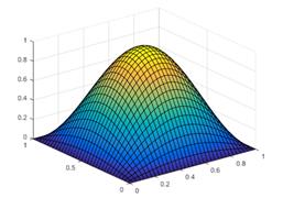
Thin circular plate bent by pressure applied to one face

 

A thin circular plate, with radius R and thickness h is made from a linear elastic solid with Young’s modulus $E$ and Poisson’s ratio $\nu$, as shown in the figure.  It is subjected to a pressure $p=p_3{e}_3$ acting perpendicular to the plate, and is simply supported at its edge.  Show that the deflection of the plate is

$u_3=\frac{3(1-{\nu }^2)p}{16E(1+\nu )h^3}\left(R^2-r^2\right)\left((5+\nu )R^2-(1+\nu )r^2\right)$

The solution should depend only on r (and not $\theta$ ) so we the differential equation for the deflection is

$\frac{E{h}^3}{12(1-{\nu }^2)}{\left(\frac{{\partial }^2}{\partial r^2}+\frac{1}{r}\frac{\partial }{\partial r}\right)}^2{u}_3=p_3$

It is tempting to solve this with MATLAB, but interestingly MATLAB returns an incorrect solution to this particular ODE at the time of writing these notes (July 2018).  So we have to do it by hand instead.  Expand out the derivatives and rearrange to get

$\frac{E{h}^3}{12(1-{\nu }^2)}\left(\frac{d^4{u}_3}{d{r}^4}+\frac{2}{r}\frac{d^3{u}_3}{d{r}^3}-\frac{1}{r^2}\frac{d^2{u}_3}{d{r}^2}+\frac{1}{r^3}\frac{d{u}_3}{dr}\right)=\frac{E{h}^3}{12(1-{\nu }^2)}\frac{1}{r}\frac{d}{dr}\left(r\frac{d}{dr}\left(\frac{1}{r}\frac{d}{dr}\left(r\frac{d{u}_3}{dr}\right)\right)\right)=p$

We can now just integrate

$u_3=\frac{1-{\nu }^2}{E{h}^3}\left(\frac{3}{16}p{r}^4+A{r}^2\log r+B\log r+C{r}^2+D\right)$

The four constants must be determined from the boundary conditions.   Note that:

1. Note that log(r) is infinite (and negative) at r=0.  But the displacement can’t be infinite!  This means B=0 .
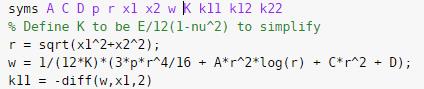
2. Now let’s find the curvature of the plate.   We can safely use MATLAB to do this.  Recall that

${\kappa }_{11}=-\frac{{\partial }^2{u}_3}{\partial x_1^2}{\kappa }_{12}={\kappa }_{21}=-\frac{{\partial }^2{u}_3}{\partial x_1\partial x_2}{\kappa }_{22}=-\frac{{\partial }^2{u}_3}{\partial x_2^2}$

For example here’s the calculation of ${\kappa }_{11}$ 

 

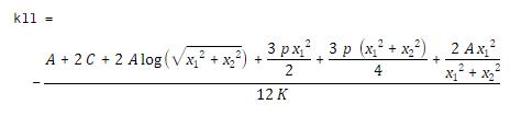
Notice that there’s a term $A\log (r)$  in the solution.   Since the curvature can’t be infinite, we see that A=0.

3. The last two boundary conditions are zero displacement $u_3=0$ and zero moment about the circumference of the plate $M_{11}{n}_1^2+2M_{12}{n}_1{n}_2+M_{22}{n}_2^2=0$ at r=R, where $n_1=x_1/R$ and $n_2=x_2/R$ are components of a unit vector perpendicular to the edge of the plate.   This gives two equations for the remaining unknown constants C and D.   MATLAB can solve the equations:

 

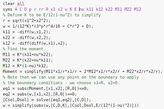
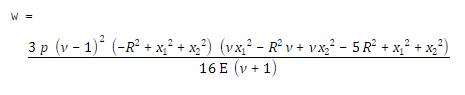
This clearly reduces to the required answer.   Note that the MATLAB script will also tell you the internal moments in the plate, if you care…