Vectors and Tensor Operations in Polar Coordinates
Many
simple boundary value problems in solid mechanics (such as those that tend to
appear in homework assignments or examinations!) are most conveniently solved
using spherical or cylindrical-polar coordinate systems.
The
main drawback of using a polar coordinate system is that there is no convenient
way to express the various vector and tensor operations using index notation everything has to be written out in
long-hand. In this section, therefore,
we completely abandon index notation vector and tensor components are always
expressed as matrices.
Spherical-polar coordinates
1.1 Specifying points in spherical-polar
coordinates
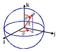 To specify points in space using spherical-polar
coordinates, we first choose two convenient, mutually perpendicular reference
directions (i and k in the picture). For example, to specify position on the
Earth’s surface, we might choose k
to point from the center of the earth towards the North Pole, and choose i to point from the center of the earth
towards the intersection of the equator (which has zero degrees latitude) and
the Greenwich Meridian (which has zero degrees longitude, by definition).
To specify points in space using spherical-polar
coordinates, we first choose two convenient, mutually perpendicular reference
directions (i and k in the picture). For example, to specify position on the
Earth’s surface, we might choose k
to point from the center of the earth towards the North Pole, and choose i to point from the center of the earth
towards the intersection of the equator (which has zero degrees latitude) and
the Greenwich Meridian (which has zero degrees longitude, by definition).
Then,
each point P in space is identified by three numbers, shown in the picture above. These
are not components of a vector.
In words:
R
is the distance of P from the origin
is the angle
between the k direction and OP
is the angle between the i direction and the projection of OP onto a plane through O normal
to k
By convention, we choose , and
1.2 Converting between Cartesian and
Spherical-Polar representations of points
When
we use a Cartesian basis, we identify points in space by specifying the
components of their position vector relative to the origin (x,y,z), such that When we use a spherical-polar coordinate
system, we locate points by specifying their spherical-polar coordinates
The formulas below relate
the two representations. They are
derived using basic trigonometry
1.3 Spherical-Polar representation of vectors
When
we work with vectors in spherical-polar coordinates, we abandon the {i,j,k} basis. Instead, we specify vectors as components in
the basis shown in the figure. For example, an arbitrary vector a is written as ,
where denote the components of a.
The basis is different for
each point P. In words
points along OP
is tangent to a line of constant longitude
through P
is tangent to a line of constant latitude
through P.
For
example if polar-coordinates are used to specify points on the Earth’s
surface, you can visualize the basis
vectors like this. Suppose you stand at
a point P on the Earths surface.
Relative to you: points vertically upwards; points due South; and points due East. Notice that the basis vectors
depend on where you are standing.
You
can also visualize the directions as follows.
To see the direction of ,
keep and fixed, and increase R. P is moving parallel to . To see the direction of ,
keep R and fixed, and increase .
P now moves parallel to . To see the direction of ,
keep R and fixed, and increase . P now moves parallel to . Mathematically, this concept can be expressed
as follows. Let r be the position vector of P.
Then
By
definition, the `natural basis’ for a coordinate system is the derivative of
the position vector with respect to the three scalar coordinates that are used
to characterize position in space (see Chapter 10 for a more detailed
discussion). The basis vectors for a
polar coordinate system are parallel to the natural basis vectors, but are
normalized to have unit length. In
addition, the natural basis for a polar coordinate system happens to be orthogonal.
Consequently, is an orthonormal basis (basis vectors have
unit length, are mutually perpendicular and form a right handed triad)
1.4
Converting vectors between Cartesian and Spherical-Polar bases
Let
be a vector, with components in the spherical-polar basis . Let denote the components of a in the basis {i,j,k}.
The two sets of components
are related by
while the inverse
relationship is
Observe
that the two 3x3 matrices involved in this transformation are transposes (and
inverses) of one another. The
transformation matrix is therefore orthogonal, satisfying ,
where denotes the 3x3 identity matrix.
Derivation: It is easiest to do the transformation by expressing
each basis vector as components in {i,j,k}, and then substituting.
To do this, recall that ,
recall also the conversion
and finally recall that by
definition
Hence, substituting for x,y,z and differentiating
Conveniently we find that .
Therefore
Similarly
while ,
so that
Finally, substituting
Collecting terms in i, j
and k, we see that
This is the result stated.
To show the inverse result,
start by noting that
(where we have used ).
Recall that
Substituting, we get
Proceeding in exactly the
same way for the other two components gives the remaining expressions
Re-writing the last three
equations in matrix form gives the result stated.
1.5 Spherical-Polar representation of tensors
The
triad of vectors is an orthonormal basis (i.e. the three basis
vectors have unit length, and are mutually perpendicular). Consequently, tensors can be represented as
components in this basis in exactly the same way as for a fixed Cartesian basis
. In particular, a general second order tensor S can be represented as a 3x3 matrix
You
can think of as being equivalent to ,
as ,
and so on. All tensor operations such as addition, multiplication by a vector,
tensor products, etc can be expressed in terms of the corresponding operations
on this matrix, as discussed in Section B2 of Appendix B.
The
component representation of a tensor can also be expressed in dyadic form as
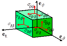 Furthermore, the physical significance of the
components can be interpreted in exactly the same way as for tensor components
in a Cartesian basis. For example, the
spherical-polar coordinate representation for the Cauchy stress tensor has the
form
Furthermore, the physical significance of the
components can be interpreted in exactly the same way as for tensor components
in a Cartesian basis. For example, the
spherical-polar coordinate representation for the Cauchy stress tensor has the
form
The component represents the traction component in direction
acting on an internal material plane with
normal ,
and so on. Of course, the Cauchy stress
tensor is symmetric, with
1.6 Constitutive equations in spherical-polar coordinates
The
constitutive equations listed in Chapter 3 all relate some measure of stress in
the solid (expressed as a tensor) to some measure of local internal deformation
(deformation gradient, Eulerian strain, rate of deformation tensor, etc), also
expressed as a tensor. The constitutive
equations can be used without modification in spherical-polar coordinates, as
long as the matrices of Cartesian components of the various tensors are
replaced by their equivalent matrices in spherical-polar coordinates.
For
example, the stress-strain relations for an isotropic, linear elastic material
in spherical-polar coordinates read
HEALTH WARNING: If you are solving a problem involving anisotropic materials using
spherical-polar coordinates, it is important to remember that the orientation
of the basis vectors vary with position. For example, for an anisotropic, linear
elastic solid you could write the constitutive equation as
however,
the elastic constants would need to be represent the material
properties in the basis ,
and would therefore be functions of position (you would have to calculate them
using the lengthy basis change formulas listed in Section 3.2.11). In practice the results are so complicated
that there would be very little advantage in working with a spherical-polar
coordinate system in this situation.
1.7 Converting tensors between Cartesian and
Spherical-Polar bases
Let
S be a tensor, with components
in
the spherical-polar basis and the Cartesian basis {i,j,k}, respectively. The
two sets of components are related by
These
results follow immediately from the general basis change formulas for tensors .
1.8 Vector Calculus using Spherical-Polar Coordinates
Calculating
derivatives of scalar, vector and tensor functions of position in
spherical-polar coordinates is complicated by the fact that the basis vectors
are functions of position. The results
can be expressed in a compact form by defining the gradient operator, which, in spherical-polar coordinates, has the
representation
In addition, the
derivatives of the basis vectors are
You can derive these
formulas by differentiating the expressions for the basis vectors in terms of {i,j,k}
and
evaluating the various derivatives. When differentiating, note that {i,j,k} are fixed, so their derivatives
are zero. The details are left as an
exercise.
The various derivatives of
scalars, vectors and tensors can be expressed using operator notation as
follows.
Gradient of a scalar function: Let denote a scalar function of position. The gradient of f is denoted by
Alternatively, in matrix
form
Gradient of a vector function Let be a vector function of position. The gradient
of v is a tensor, which can be
represented as a dyadic product of the vector with the gradient operator as
The
dyadic product can be expanded but when evaluating the derivatives it is
important to recall that the basis vectors are functions of the coordinates and consequently their derivatives do not
vanish. For example
Verify for yourself that
the matrix representing the components of the gradient of a vector is
Divergence of a vector function Let be a vector function of position. The
divergence of v is a scalar, which
can be represented as a dot product of the vector with the gradient operator as
Again,
when expanding the dot product, it is important to remember to differentiate
the basis vectors. Alternatively, the divergence can be expressed as ,
which immediately gives
Curl of a vector function Let be a vector function of position. The curl of v is a vector, which can be represented
as a cross product of the vector with the gradient operator as
The curl rarely appears in
solid mechanics so the components will not be expanded in full
Divergence of a tensor function. Let be a tensor, with dyadic representation
The divergence of S is a vector, which can be represented
as
Evaluating
the components of the divergence is an extremely tedious operation, because
each of the basis vectors in the dyadic representation of S must be differentiated, in addition to the components
themselves. The final result (expressed
as a column vector) is
2: Cylindrical-polar coordinates
2.1 Specifying points in space using in cylindrical-polar
coordinates
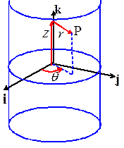
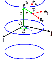
To
specify the location of a point in cylindrical-polar coordinates, we choose an
origin at some point on the axis of the cylinder, select a unit vector k to be parallel to the axis of the
cylinder, and choose a convenient direction for the basis vector i, as shown in the picture. We then use the three numbers to locate a point inside the cylinder, as
shown in the picture. These are not components of a vector.
In words
r is the radial distance of P from the axis of the cylinder
is the angle
between the i direction and the projection of OP onto the i,j plane
z
is the length of the projection of OP on the axis of the cylinder.
By convention r>0 and
2.2 Converting between cylindrical polar and
rectangular cartesian coordinates
When
we use a Cartesian basis, we identify points in space by specifying the
components of their position vector relative to the origin (x,y,z), such that When we use a spherical-polar coordinate
system, we locate points by specifying their spherical-polar coordinates
The formulas below relate
the two representations. They are
derived using basic trigonometry
 2.3
Cylindrical-polar representation of vectors
2.3
Cylindrical-polar representation of vectors
When
we work with vectors in spherical-polar coordinates, we specify vectors as
components in the basis shown in the figure. For example, an arbitrary vector a is written as ,
where denote the components of a.
The
basis vectors are selected as follows
is a unit vector normal to the cylinder at P
is a unit vector circumferential to the
cylinder at P, chosen to make a right handed triad
is parallel to the k vector.
You will see that the
position vector of point P would be expressed as
Note also that the basis
vectors are intentionally chosen to satisfy
The
basis vectors have unit length, are mutually perpendicular, and form a right
handed triad and therefore is an orthonormal basis. The basis vectors are parallel to (but not
equivalent to) the natural basis vectors for a cylindrical polar coordinate
system (see Chapter 10 for a more detailed discussion).
2.4 Converting vectors between Cylindrical and Cartesian
bases
Let
be a vector, with components in the spherical-polar basis . Let denote the components of a in the basis {i,j,k}.
The two sets of components
are related by
Observe
that the two 3x3 matrices involved in this transformation are transposes (and
inverses) of one another. The
transformation matrix is therefore orthogonal, satisfying ,
where denotes the 3x3 identity matrix.
The
derivation of these results follows the procedure outlined in E.1.4 exactly,
and is left as an exercise.
2.5 Cylindrical-Polar representation of tensors
The
triad of vectors is an orthonormal basis (i.e. the three basis
vectors have unit length, and are mutually perpendicular). Consequently, tensors can be represented as
components in this basis in exactly the same way as for a fixed Cartesian basis
. In particular, a general second order tensor S can be represented as a 3x3 matrix
You
can think of as being equivalent to ,
as ,
and so on. All tensor operations such as addition, multiplication by a vector,
tensor products, etc can be expressed in terms of the corresponding operations
on this matrix, as discussed in Section B2 of Appendix B.
The
component representation of a tensor can also be expressed in dyadic form as
The
remarks in Section E.1.5 regarding the physical significance of tensor
components also applies to tensor components in cylindrical-polar coordinates.
2.6 Constitutive equations in cylindrical-polar
coordinates
The
constitutive equations listed in Chapter 3 all relate some measure of stress in
the solid (expressed as a tensor) to some measure of local internal deformation
(deformation gradient, Eulerian strain, rate of deformation tensor, etc), also
expressed as a tensor. The constitutive
equations can be used without modification in cylindrical-polar coordinates, as
long as the matrices of Cartesian components of the various tensors are
replaced by their equivalent matrices in spherical-polar coordinates.
For
example, the stress-strain relations for an isotropic, linear elastic material
in cylindrical-polar coordinates read
The
cautionary remarks regarding anisotropic materials in E.1.6 also applies to
cylindrical-polar coordinate systems.
2.7 Converting tensors between Cartesian and
Spherical-Polar bases
Let
S be a tensor, with components
in
the cylindrical-polar basis and the Cartesian basis {i,j,k}, respectively. The
two sets of components are related by
2.8 Vector Calculus using Cylindrical-Polar
Coordinates
Calculating
derivatives of scalar, vector and tensor functions of position in
cylindrical-polar coordinates is complicated by the fact that the basis vectors
are functions of position. The results
can be expressed in a compact form by defining the gradient operator, which, in spherical-polar coordinates, has the
representation
In addition, the nonzero derivatives
of the basis vectors are
The various derivatives of
scalars, vectors and tensors can be expressed using operator notation as
follows.
Gradient of a scalar function: Let denote a scalar function of position. The gradient of f is denoted by
Alternatively, in matrix
form
Gradient of a vector function Let be a vector function of position. The gradient
of v is a tensor, which can be
represented as a dyadic product of the vector with the gradient operator as
The
dyadic product can be expanded but when evaluating the derivatives it is
important to recall that the basis vectors are functions of the coordinate and consequently their derivatives may not
vanish. For example
Verify for yourself that
the matrix representing the components of the gradient of a vector is
Divergence of a vector function Let be a vector function of position. The
divergence of v is a scalar, which
can be represented as a dot product of the vector with the gradient operator as
Again,
when expanding the dot product, it is important to remember to differentiate
the basis vectors. Alternatively, the divergence can be expressed as ,
which immediately gives
Curl of a vector function Let be a vector function of position. The curl of v is a vector, which can be represented
as a cross product of the vector with the gradient operator as
The curl rarely appears in
solid mechanics so the components will not be expanded in full
Divergence of a tensor function. Let
be a tensor, with dyadic representation
The divergence of S is a vector, which can be represented
as
Evaluating
the components of the divergence is an extremely tedious operation, because
each of the basis vectors in the dyadic representation of S must be differentiated, in addition to the components
themselves. The final result (expressed
as a column vector) is