Chapter 4
Conservation laws for systems of
particles
In this chapter, we shall
introduce the following general concepts:
- The power, or rate of work done by a force
- The total work done by a force
- The kinetic energy of a particle
- The power-kinetic energy and work-kinetic energy
relations for a single particle
- The concepts of a conservative force and a conservative
system
- The power-total energy and work-total energy
relations for a conservative system
- Energy conservation for a conservative system
- The linear impulse of a force
- The linear momentum of a particle (or system of
particles)
- The linear impulse - linear momentum relations
for a single particle
- Linear impulse-momentum relations for a system of
particles
- Conservation of linear momentum for a system
- Analyzing collisions between particles using
linear momentum
- The angular impulse of a force
- The angular momentum of a particle
- The angular impulse angular momentum relation for a single
particle
We
will also illustrate how these concepts can be used in engineering
calculations. As you will see, to applying
these principles to engineering calculations you will need two things: (i) a
thorough understanding of the principles themselves; and (ii) Physical insight
into how engineering systems behave, so you can see how to apply the theory to
practice. The first is easy. The second is hard, but practice will help.
4.1 Work, Power, Potential Energy and Kinetic Energy
relations for particles
The
concepts of work, power and energy are among the most powerful ideas in the
physical sciences. Their most important
application is in the field of thermodynamics,
which describes the exchange of energy between interacting systems. In addition, concepts of energy carry over to
relativistic systems and quantum mechanics, where the classical versions of Newton’s laws
themselves no longer apply.
In this section, we develop
the basic definitions of mechanical work and energy, and show how they can be
used to analyze motion of dynamical systems.
Future courses will expand on these concepts further.
4.1.1 Definition of the power and work done by a force
Suppose that a force F acts on a particle that moves with
speed v.
By definition:
 The Power
developed by the force, (or the rate of
work done by the force) is .
The Power
developed by the force, (or the rate of
work done by the force) is .
If
both force and velocity are expressed in Cartesian components, then
Power
has units of Nm/s, or `Watts’ in SI units.
 The work done by the force during a time interval is
The
work done by the force can also be calculated by integrating the force vector
along the path traveled by the force, as
where
are the initial and final positions of the
force.
Work
has units of Nm in SI units, or `Joules’
A
moving force can do work on a particle, or on any moving object. For example, if a force acts to stretch a
spring, it is said to do work on the spring.
4.1.2 Simple examples of power and work calculations
 Example 1: An aircraft with mass 45000 kg flying at 200 knots
(102m/s) climbs at 1000ft/min. Calculate
the rate of work done on the aircraft by gravity.
Example 1: An aircraft with mass 45000 kg flying at 200 knots
(102m/s) climbs at 1000ft/min. Calculate
the rate of work done on the aircraft by gravity.
The gravitational force is ,
and the velocity vector of the aircraft is . The rate of work done on the aircraft is
therefore
Substituting numbers gives
 Example 2:
Calculate a formula for the work required to
stretch a spring with stiffness k and
unstretched length from length to length .
Example 2:
Calculate a formula for the work required to
stretch a spring with stiffness k and
unstretched length from length to length .
The
figure shows a spring that held fixed at A
and is stretched in the horizontal direction by a force acting at B. At some instant the spring has length . The spring force law states that the force
acting on the spring at B is related to the length of the spring x by
The position vector of the
force is ,
and therefore the work done is
 Example 3:
Calculate the work done by gravity on a
satellite that is launched from the surface of the earth to an altitude of
250km (a typical low earth orbit).
Example 3:
Calculate the work done by gravity on a
satellite that is launched from the surface of the earth to an altitude of
250km (a typical low earth orbit).
Assumptions
- The earth’s radius is 6378.145km
- The mass of a typical satellite is 4135kg - see , e.g. http://www.astronautix.com/craft/hs601.htm
- The Gravitational parameter (G=
gravitational constant; M=mass
of earth)
- We will assume that
the satellite is launched along a straight line path parallel to the i direction, starting the earths
surface and extending to the altitude of the orbit. It turns out that the work done is
independent of the path, but this is not obvious without more elaborate
and sophisticated calculations.
Calculation:
- The gravitational force on the satellite is
- The work done follows as
- Substituting numbers gives J (be careful with units if you work with kilometers the work done
is in N-km instead of SI units Nm)
 Example 4: A Ferrari Testarossa skids to a stop over a distance
of 250ft. Calculate the total work done
on the car by the friction forces acting on its wheels.
Example 4: A Ferrari Testarossa skids to a stop over a distance
of 250ft. Calculate the total work done
on the car by the friction forces acting on its wheels.
Assumptions:
- A Ferrari Testarossa has mass 1506kg (see http://www.ultimatecarpage.com/car/1889/Ferrari-Testarossa.html)
- The coefficient of friction between wheels and
road is of order 0.8
- We assume the brakes are locked so all wheels
skid, and air resistance is neglected
Calculation The figure shows a free body diagram. The equation of
motion for the car is
- The vertical component of the equation of motion
yields
- The friction law shows that
- The position vectors of the car’s front and rear
wheels are . The work
done follows as. We suppose that
the rear wheel starts at some point when the
brakes are applied and skids a total distance d.
- The work done follows as . Substituting
numbers gives .
 Example 5: The figure shows a box that is pushed up a slope by a
force P. The box moves with speed v. Find a formula for the rate of work done by each of the forces
acting on the box.
Example 5: The figure shows a box that is pushed up a slope by a
force P. The box moves with speed v. Find a formula for the rate of work done by each of the forces
acting on the box.
The figure shows a free body
diagram. The force vectors are
1.
Applied force
2.
Friction
3.
Normal reaction
4.
Weight
 The velocity vector is
Evaluating the dot products for each
formula, and recalling that gives
1.
Applied force
2.
Friction
3.
Normal reaction
4.
Weight
|
Force
N
|
Draw
(cm)
|
|
0
|
0
|
|
40
|
10
|
|
90
|
20
|
|
140
|
30
|
|
180
|
40
|
|
220
|
50
|
|
270
|
60
|
Example 6: The
table lists the experimentally measured force-v-draw data for a long-bow. Calculate the total work done to draw the
bow.
In
this case we don’t have a function that specifies the force as a function of
position; instead, we have a table of numerical values. We have to approximate the integral
numerically. To understand how to do this, remember that
integrating a function can be visualized as computing the area under a curve of
the function, as illustrated in the figure.
 We can estimate the integral by dividing the area into
a series of trapezoids, as shown. Recall
that the area of a trapezoid is (base x average height), so the total area of
the function is
We can estimate the integral by dividing the area into
a series of trapezoids, as shown. Recall
that the area of a trapezoid is (base x average height), so the total area of
the function is
You could easily do this
calculation by hand but for lazy people like me MATLAB has a
convenient function called `trapz’ that does this calculation
automatically. Here’s how to use it
draw = [0,10,20,30,40,50,60]*0.01;
force = [0,40,90,140,180,220,270];
trapz(draw,force)
ans = 80.5000
So the solution is 80.5J
 4.1.3 Definition
of the potential energy of a conservative force
4.1.3 Definition
of the potential energy of a conservative force
Preamble: Textbooks nearly always define the `potential energy
of a force.’ Strictly speaking, we
cannot define a potential energy of a single force instead, we need to define the potential
energy of a pair of forces. A force
can’t exist by itself there must always be an equal and opposite
reaction force acting on a second body.
In all of the discussion to be presented in this section, we
implicitly assume that the reaction force is acting on a second body, which is
fixed at the origin. This
simplifies calculations, and makes the discussion presented here look like
those given in textbooks, but you should remember that the potential energy of
a force pair is always a function of the relative positions of the two forces.
With that proviso, consider a
force F acting on a particle at some
position r in space. Recall that the
work done by a force that moves from position vector to position vector is
In general, the work done by
the force depends on the path between to . For some special forces, however, the work
done is independent of the path. Such
forces are said to be conservative.
For
a force to be conservative:
The force must be a function only of its
position i.e. it can’t depend on the velocity of the
force, for example.
The force vector must satisfy
Examples
of conservative forces include gravity, electrostatic forces, and the forces
exerted by a spring. Examples of non-conservative
(or should that be liberal?) forces include friction, air resistance, and
aerodynamic lift forces.
The
potential
energy of a conservative force is defined as the negative of the work
done by the force in moving from some arbitrary initial position to a new position ,
i.e.
The
constant is arbitrary, and the negative sign is introduced by convention (it
makes sure that systems try to minimize their potential energy). If there is a point where the force is zero,
it is usual to put at this point, and take the constant to be
zero.
Note that
- The potential energy is a scalar valued function
- The potential energy
is a function only of the position of the force. If we choose to describe position in
terms of Cartesian components ,
then .
- The relationship between potential energy and
force can also be expressed in differential
form (which is often more useful for actual calculations) as
If
we choose to work with Cartesian components, then
Occasionally,
you might have to calculate a potential energy function by integrating forces for example, if you are interested in running a molecular
dynamic simulation of a collection of atoms in a material, you will need to describe
the interatomic forces in some convenient way.
The interatomic forces can be estimated by doing quantum-mechanical
calculations, and the results can be approximated by a suitable potential
energy function. Here are a few examples
showing how you can integrate forces to calculate potential energy
 Example 1: Potential energy of forces exerted by a
spring. A free body diagram showing the forces
exerted by a spring connecting two objects is shown in the figure.
Example 1: Potential energy of forces exerted by a
spring. A free body diagram showing the forces
exerted by a spring connecting two objects is shown in the figure.
- The force exerted by a
spring is
- The position vector of the force is
- The potential energy follows as
where we have taken the constant to be zero.
Example
2: Potential energy of electrostatic forces exerted by charged particles.
The
figure shows two charged particles a distance x apart. To calculate the
potential energy of the force acting on particle 2, we place particle 1 at the
origin, and note that the force acting on particle 2 is
where
and are the charges on the two particles, and is a fundamental physical constant known as
the Permittivity of the medium
surrounding the particles. Since the
force is zero when the particles are infinitely far apart, we take at infinity.
The potential energy follows as
Table
of potential energy relations
In
practice, however, we rarely need to do the integrals to calculate the potential
energy of a force, because there are very few different kinds of force. For most engineering calculations the
potential energy formulas listed in the table below are sufficient.
|
Type of force
|
Force vector
|
Potential energy
|
|
|
Gravity acting on a particle near earths surface
|
|
|
|
|
Gravitational force exerted on mass m by mass M at the
origin
|
|
|
|
|
Force exerted by a spring with stiffness k and unstretched length
|
|
|
|
|
Force acting between two charged particles
|
|
|
|
|
Force exerted by one molecule of a noble gas (e.g. He, Ar,
etc) on another (Lennard Jones potential). a is the equilibrium spacing between molecules, and E is the energy of the bond.
|
|
|
|
 4.1.4
Definition of the Kinetic Energy of a particle
4.1.4
Definition of the Kinetic Energy of a particle
Consider a particle with mass
m which moves with velocity . By definition, its kinetic energy is
|
|
|
|
4.1.5 Power-Work-kinetic energy relations
for a single particle
Consider
a particle with mass m that moves
under the action of a force F. Suppose
that
- At some time the particle has some initial position ,
velocity and kinetic energy
- At some later time the particle has a new position r, velocity and kinetic energy .
- Let denote the rate of work done by the force
- Let be the total work done by the force
The
Power-kinetic energy relation for the
particle states that the rate of work done by F is equal to the rate of change of kinetic energy of the particle,
i.e.
|
|
|
|
Proof: This is just another way of writing Newton’s law for
the particle: to see this, note that we can take the dot product of both sides
of F=ma with the particle velocity
|
|
|
|
To see the last step, do the
derivative using the Chain rule and note that .
The
Work-kinetic energy relation for a
particle says that the total work done by the force F on the particle is equal to the change in the kinetic energy of
the particle.
This follows by integrating
the power-kinetic energy relation with respect to time.
4.1.6 Examples of simple calculations using
work-power-kinetic energy relations
There
are two main applications of the work-power-kinetic energy relations. You can use them to calculate the distance
over which a force must act in order to produce a given change in velocity. You can also use them to estimate the energy
required to make a particle move in a particular way, or the amount of energy
that can be extracted from a collection of moving particles (e.g. using a wind
turbine)
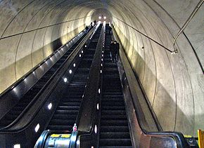 Example 1: The longest single-span escalator in the Western
hemisphere is located at the Washington Metro station in Montgomery County,
Maryland. Some technical specifications
for the escalator span can be found on Wikipedia (we
have not checked this data!).
Additional information concerning escalator standards can be found here.
Example 1: The longest single-span escalator in the Western
hemisphere is located at the Washington Metro station in Montgomery County,
Maryland. Some technical specifications
for the escalator span can be found on Wikipedia (we
have not checked this data!).
Additional information concerning escalator standards can be found here.
Calculate
the kinetic energy of a single 80kg rider standing on the escalator
The KE is ;
we have that the speed is 27m per minute, so KE is 8.1J.
Calculate
the change in potential energy of a single 80kg rider who travels the entire
length of the escalator span.
The change in PE is mgh, where h = 35m , so PE is 27468J
Assuming
the escalator operates at its theoretical capacity of 9000 passengers per hour,
estimate the power required to operate the escalator.
The power is the number of passengers per second
multiplied by the energy change per passenger.
This gives P=68.7 kW
Example 2: Estimate the minimum distance required for a 14
wheeler that travels at the RI speed-limit to brake to a standstill. Is the distance to stop any different for a
Toyota Echo?
This
problem can be solved by noting that, since we know the initial and final speed
of the vehicle, we can calculate the change in kinetic energy as the vehicle
stops. The change in kinetic energy must
equal the work done by the forces acting on the vehicle which depends on the distance slid. Here are the details of the calculation.
 Assumptions:
- We assume that all the
wheels are locked and skid over the ground (this will stop the vehicle in
the shortest possible distance)
- The contacts are
assumed to have friction coefficient
- The vehicle is
idealized as a particle.
- Air resistance will be
neglected.
Calculation:
- The figure shows a
free body diagram.
- The equation of motion
for the vehicle is
The vertical component of the equation shows that .
- The friction force
follows as
- If the vehicle skids
for a distance d, the total work
done by the forces acting on the vehicle is
- The work-energy relation states that the total
work done on the particle is equal to its change in kinetic energy. When the brakes are applied the vehicle
is traveling at the speed limit, with speed V; at the end of the skid its speed is zero. The change in kinetic energy is
therefore . The
work-energy relation shows that
Substituting numbers gives
This
simple calculation suggests that the braking distance for a vehicle depends
only on its speed and the friction coefficient between wheels and tires. This is unlikely to vary much from one
vehicle to another. In practice there
may be more variation between vehicles than this estimate suggests, partly
because factors like air resistance and aerodynamic lift forces will influence
the results, and also because vehicles usually don’t skid during an emergency
stop (if they do, the driver loses control) the nature of the braking system therefore
also may change the prediction.
Example 3: Compare the power consumption of a Ford Excursion to
that of a Chevy Cobalt during stop-start driving in a traffic jam.
During
stop-start driving, the vehicle must be repeatedly accelerated to some (low)
velocity; and then braked to a stop. Power is expended to accelerate the
vehicle; this power is dissipated as heat in the brakes during braking. To calculate the energy consumption, we must
estimate the energy required to accelerate the vehicle to its maximum speed,
and estimate the frequency of this event.
Calculation/Assumptions:
- We assume that the
speed in a traffic jam is low enough that air resistance can be neglected.
- The energy to
accelerate to speed V is .
- We assume that the
vehicle accelerates and brakes with constant acceleration if so, its average speed is V/2.
- If the vehicle travels
a distance d between stops, the
time between two stops is 2d/V.
- The average power is
therefore .
- Taking V=15mph (7m/s) and d=200ft (61m) are reasonable values
the power is therefore 0.03m, with m in kg. A Ford Excursion weighs 9200 lb (4170
kg), requiring 125 Watts (about that of a light bulb) to keep moving. A Chevy Cobalt weighs 2681lb (1216kg)
and requires only 36 Watts a very substantial energy saving.
Reducing
vehicle weight is the most effective way of improving fuel efficiency during
slow driving, and also reduces manufacturing costs and material requirements. Another, more costly, approach is to use a
system that can recover the energy during braking this is the main reason that hybrid vehicles
like the Prius have better fuel economy than conventional vehicles.
 Example 4: Estimate the power that can be generated by a wind
turbine.
Example 4: Estimate the power that can be generated by a wind
turbine.
The
figure shows a wind turbine. The turbine
blades deflect the air flowing past them: this changes the air speed and so
exerts a force on the blades. If the
blades move, the force exerted by the air on the blades does work this work is the power generated by the
turbine. The rate of work done by the
air on the blades must equal the change in kinetic energy of the air as it
flows past the blades. Consequently, we
can estimate the power generated by the turbine by calculating the change in
kinetic energy of the air flowing through it.
To
do this properly needs a very sophisticated analysis of the air flow around the
turbine. However, we can get a rather
crude estimate of the power by assuming that the turbine is able to extract all
the energy from the air that flows through the circular area swept by the blades.
Calculation: Let V
denote the wind speed, and let denote the density of the air.
1. In a time t,
a cylindrical region of air with radius R
and height Vt passes through the fan.
2. The cylindrical region has mass
3. The kinetic energy of the cylindrical region of air is
4. The rate of flow of kinetic energy through the fan is
therefore
5. If all this energy could be used to do work on the fan
blades the power generated would be
Representative
numbers are (i) Air density 1.2 ;
(ii) air speed 25mph (11 m/sec); (iii) Radius 30m
This
gives 1.8MW. For comparison, a nuclear power plant
generates about 500-1000 MW.
A
more sophisticated calculation (which will be covered in EN810) shows that in
practice the maximum possible amount of energy that can be extracted from the
air is about 60% of this estimate. On
average, a typical household uses about a kW of energy; so a single turbine
could provide enough power for about 5-10 houses.
4.1.7 Energy relations for a
conservative system of particles.
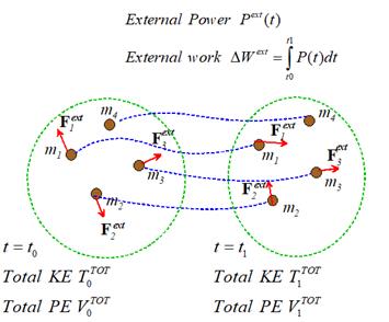
 The figure shows a `system of particles’ this is just a collection of objects that we
might be interested in, which can be idealized as particles. Each particle in the system can
experience forces applied by:
The figure shows a `system of particles’ this is just a collection of objects that we
might be interested in, which can be idealized as particles. Each particle in the system can
experience forces applied by:
Other particles in the system (e.g.
due to gravity, electric charges on the particles, or because the particles are
physically connected through springs, or because the particles collide). We call these internal forces acting in
the system. We will denote the internal
force exerted by the ith particle on
the jth particle by . Note that, because every action has an equal
and opposite reaction, the force exerted on the jth particle by the ith
particle must be equal and opposite, to ,
i.e. .
Forces exerted on the particles by the
outside world (e.g. by externally applied gravitational or
electromagnetic fields, or because the particles are connected to the outside
world through mechanical linkages or springs).
We call these external forces acting on the
system, and we will denote the external force on the i th particle by
We
define the rate of external work (or
external power) done on the system as
We
define the total external work done on
the system during a time interval as the sum of the work done by the external
forces.
The
total work done can also include a contribution from external moments acting on
the system, but we will worry about this when we analyze rigid body motion..
The
system of particles is conservative if all the internal
forces in the system are conservative.
This means that the particles must interact through conservative forces
such as gravity, springs, electrostatic forces, and so on. The particles can also be connected by rigid
links, or touch one another, but contacts between particles must be
frictionless.
If
this is the case, we can define the total
potential energy of the system as the sum of potential energies of all the
internal forces. We usually compute
the total potential energy by summing up all the terms from the table in Sect
4.1.3. Mathematically, the potential
energy depends in some complicated way on the distances between all the
particles, and the resultant force on the ith
particle is related to the total potential energy by
We
also define the total kinetic energy of the system as the sum of kinetic energies
of all the particles.
The
work-energy relation for the system of particles can then be stated as
follows. Suppose that
- At some time the system has and kinetic energy
- At some later time the system has kinetic energy .
- Let denote the potential energy of the force
at time
- Let denote the potential energy of the force
at time
- Let denote the total work done on the system
between
Power
Energy Relation: This law states
that the rate of external work done on the system is equal to the rate of
change of total energy of the system
Work
Energy Relation: This law states
that the external work done on the system is equal to the change in total
kinetic and potential energy of the system.
Energy conservation law For the special case where no external forces act on the
system, the total energy of the system is
constant
It
is worth making one final remark before we turn to applications of these laws. We often invoke the principle of conservation
of energy when analyzing the motion of an object that is subjected to the
earth’s gravitational field. For
example, the first problem we solve in the next section involves the motion of
a projectile launched from the earth’s surface.
We usually glibly say that `the sum of the potential and kinetic
energies of the particle are constant’ and if you’ve done physics courses you’ve
probably used this kind of thinking. It
is not really correct, although it leads to a more or less correct solution.
Properly,
we should consider the earth and the projectile together as a conservative
system. This means we must include the
kinetic energy of the earth in the calculation, which changes by a small, but
finite, amount due to gravitational interaction with the projectile. Fortunately, the principle of conservation
of linear momentum (to be covered later) can be used to show that the change in
kinetic energy of the earth is negligibly small compared to that of the
particle.
Proof of the energy relation
Recall the power-kinetic energy
relation for a single particle
The total force on one
particle consists of the external force, plus the sum of all the forces exerted
on the particle by other particles. The
power-energy relation for the i th
particle therefore becomes
Since the internal forces are
conservative, we can write
Furthermore, , so that
We can now sum this over all
the particles
We know that depends only on the positions of the
particles, so the second term on the left hand side is a total differential
(by the chain rule). We also recognize the first term as the
total external power, and the right hand side as the time derivative of the
total KE, so we see that
Rearranging this gives the
power-KE relation for the system, and integrating it with respect to time gives
the work-energy relation.
4.1.8 Examples of calculations using
kinetic and potential energy in conservative systems
The kinetic-potential energy
relations can be used to quickly calculate relationships between the velocity
and position of an object. Several
examples are provided below.
Example 1: (Boring FE exam question) A projectile with mass m is launched from the ground with velocity at angle . Calculate an expression for the maximum
height reached by the projectile.
If
air resistance can be neglected, we can regard the earth and the projectile
together as a conservative system. We neglect the change in the earth’s kinetic
energy. In addition, since the gravitational force acting on the particle is
vertical, the particle’s horizontal component of velocity must be
constant.
Calculation:
- Just after launch, the velocity of the particle
is
- The kinetic energy of the particle just after
launch is .
Its potential energy is zero.
- At the peak of the trajectory the vertical
velocity is zero. Since the horizontal velocity remains constant, the
velocity vector at the peak of the trajectory is .
The kinetic energy at this point is therefore
- Energy is conserved, so
 Example 2: You are asked to design the packaging for a sensitive
instrument. The packaging will be made
from an elastic foam, which behaves like a spring. The specifications restrict
the maximum acceleration of the instrument to 15g. Estimate the thickness of the packaging that
you must use.
Example 2: You are asked to design the packaging for a sensitive
instrument. The packaging will be made
from an elastic foam, which behaves like a spring. The specifications restrict
the maximum acceleration of the instrument to 15g. Estimate the thickness of the packaging that
you must use.
This
problem can be solved by noting that (i) the max acceleration occurs when the
packaging (spring) is fully compressed and so exerts the maximum force on the
instrument; (ii) The velocity of the instrument must be zero at this instant,
(because the height is a minimum, and the velocity is the derivative of the height);
and (iii) The system is conservative, and has zero kinetic energy when the
package is dropped, and zero kinetic energy when the spring is fully
compressed.
Assumptions:
- The package is dropped
from a height of 1.5m
- The effects of air
resistance during the fall are neglected
- The foam is idealized
as a linear spring, which can be fully compressed.
Calculations:
Let h denote the drop height; let d
denote the foam thickness.
- The potential energy
of the system just before the package is dropped is mgh
- The potential energy
of the system at the instant when the foam is compressed to its maximum
extent is
- The total energy of
the system is constant, so
 The figure shows a free body diagram for the
instrument at the instant of maximum foam compression. The resultant force acting on the
instrument is ,
so its acceleration follows as . The acceleration must not exceed 15g, so
The figure shows a free body diagram for the
instrument at the instant of maximum foam compression. The resultant force acting on the
instrument is ,
so its acceleration follows as . The acceleration must not exceed 15g, so
- Dividing (3) by (4) shows that
The
thickness of the protective foam must therefore exceed 18.8cm.

Example 3: The Charpy
Impact Test is a way to measure the work of fracture of a material (i.e.
the work per unit area required to separate a material into two pieces). An example (from www.qualitest-inc.com/qpi.htm)
is shown in
the picture. You can see one in Prince
Lab if you are curious.
It consists of a pendulum, which swings down from a
prescribed initial angle to strike a specimen.
The pendulum fractures the specimen, and then continues to swing to a
new, smaller angle on the other side of the vertical. The scale on the pendulum allows the initial
and final angles to be measured. The
goal of this example is to deduce a relationship between the angles and the
work of fracture of the specimen.
 The figure shows the pendulum before and after it hits
the specimen.
The figure shows the pendulum before and after it hits
the specimen.
- The potential energy of the mass before it is
released is . Its kinetic energy is zero.
- The potential energy of the mass when it comes to
rest after striking the specimen is .
The kinetic energy is again zero.
The work of fracture is equal
to the change in potential energy -
Example 4: Estimate
the maximum distance that a long-bow can fire an arrow.
We
can do this calculation by idealizing the bow as a spring, and estimating the
maximum force that a person could apply to draw the bow. The
energy stored in the bow can then be estimated, and energy conservation can be
used to estimate the resulting velocity of the arrow.
Assumptions
- The long-bow will be idealized as a linear spring
- The maximum draw force is likely to be around 60lbf
(270N)
- The draw length is about 2ft (0.6m)
- Arrows come with various masses typical range is between 250-600 grains
(16-38 grams)
- We will neglect the mass of the bow (this is not
a very realistic assumption)
Calculation: The calculation needs two steps: (i) we start by
calculating the velocity of the arrow just after it is fired. This will be done
using the energy conservation law; and (ii) we then calculate the distance
traveled by the arrow using the projectile trajectory equations derived in the
preceding chapter.
- Just before the arrow is released, the spring is
stretched to its maximum length, and the arrow is stationary. The total energy of the system is ,
where L
is the draw length and k is the
stiffness of the bow.
- We can estimate values for the spring stiffness
using the draw force: we have that ,
so . Thus .
- Just after the arrow is fired, the spring returns
to its un-stretched length, and the arrow has velocity V. The total energy of the system
is ,
where m
is the mass of the arrow
- The system is conservative, therefore
- We suppose that the arrow is launched from the
origin at an angle to the
horizontal. The horizontal and vertical components of velocity are .
The position vector of the arrow can be
calculated using the method outlined in Section 3.2.2 the result is
We
can calculate the distance traveled by noting that its position vector when it
lands is di. This gives
where
t is the time of flight. The i and
j components of this equation can be
solved for t and d, with the result
The
arrow travels furthest when fired at an angle that maximizes - i.e. 45
degrees. The distance follows as
- Substituting numbers
gives 2064m for a 250 grain arrow over a mile! Of course air resistance will reduce
this value, and in practice the kinetic energy associated with the motion
of the bow and bowstring (neglected here) will reduce the distance.
 Example 5: Find a formula for the escape velocity of a space
vehicle as a function of altitude above the earths surface.
Example 5: Find a formula for the escape velocity of a space
vehicle as a function of altitude above the earths surface.
The
term ‘Escape velocity’ means that the space vehicle has a large enough velocity
to completely escape the earth’s gravitational field i.e. the space vehicle will never stop after
being launched.
Assumptions
- The space vehicle is
initially in orbit at an altitude h above
the earth’s surface
- The earth’s radius is 6378.145km
- While in orbit, a
rocket is burned on the vehicle to increase its speed to v (the escape velocity), placing it
on a hyperbolic trajectory that will eventually escape the earth’s
gravitational field.
- The Gravitational parameter (G=
gravitational constant; M=mass
of earth)
-
Calculation
- Just after the rocket
is burned, the potential energy of the system is ,
while its kinetic energy is
- When it escapes the
earth’s gravitational field (at an infinite height above the earth’s
surface) the potential energy is zero.
At the critical escape velocity, the velocity of the spacecraft at
this point drops to zero. The total
energy at escape is therefore zero.
- This is a conservative system, so
- A typical low earth
orbit has altitude of 250km. For
this altitude the escape velocity is 10.9km/sec.
4.2 Linear impulse-momentum relations
4.2.1 Definition of the linear impulse of a force
In most dynamic problems, particles are subjected to
forces that vary with time. We can write
this mathematically by saying that the force is a vector valued function of
time . If we express the force as components in a
fixed basis ,
then
where each component of the force is a function of
time.
The Linear Impulse exerted by
a force during a time interval is defined as
The linear impulse is a
vector, and can be expressed as components in a basis
If you know the force as a
function of time, you can calculate its impulse using simple calculus. For example:
1.
For a constant force, with vector value ,
the impulse is
2.
For a harmonic force of the form the impulse is
It is rather rare in
practice to have to calculate the impulse of a force from its time variation.
4.2.2 Definition of the linear momentum of a particle
The linear momentum of a
particle is simply the product of its mass and velocity
The linear momentum is a
vector its direction is parallel to the velocity of
the particle.
4.2.3 Impulse-momentum relations for a single particle
Consider a particle that is subjected to a
force for a time interval .
Let denote the impulse exerted by F on the particle
Let denote the linear momentum of the particle at
time .
Let denote the linear momentum of the particle at
time .
The
impulse-momentum equation can be expressed either in differential or integral
form.
1.
 In differential form
This
is clearly just a different way of writing Newton’s law F=ma.
2.
In integral form
This
is the integral of Newton’s
law of motion with respect to time.
The impulse-momentum
relations for a single particle are useful if you need to calculate the change
in velocity of an object that is subjected to a prescribed force.
4.2.4 Examples using impulse-momentum relations for a
single particle
 Example 1: Estimate
the time that it takes for a Ferrari Testarossa traveling at the RI speed limit
to make an emergency stop. (Like many textbook problems this one is totally
unrealistic nobody in a Ferrari is going to travel at the
speed limit!)
Example 1: Estimate
the time that it takes for a Ferrari Testarossa traveling at the RI speed limit
to make an emergency stop. (Like many textbook problems this one is totally
unrealistic nobody in a Ferrari is going to travel at the
speed limit!)
We
can do this calculation using the impulse-momentum relation for a single
particle. Assume that the car has mass m, and travels with speed V before the brakes are applied. Let denote the time required to stop.
1.  Start by estimating the force acting on the car during
an emergency stop. The figure shows a
free body diagram for the car as it brakes to a standstill. We
assume that the driver brakes hard enough to lock the wheels, so that the car
skids over the road. The horizontal
friction forces must oppose the sliding, as shown in the picture. F=ma for the car follows as
Start by estimating the force acting on the car during
an emergency stop. The figure shows a
free body diagram for the car as it brakes to a standstill. We
assume that the driver brakes hard enough to lock the wheels, so that the car
skids over the road. The horizontal
friction forces must oppose the sliding, as shown in the picture. F=ma for the car follows as
The vertical component of the equation of motion shows
that . The friction law then shows that
2.
The force acting
on the car is constant, so the impulse that brings the car to a halt is
3. The linear momentum of the car before the brakes are
applied is . The linear momentum after the car stops is
zero. Therefore, .
4.
The linear
impulse-momentum relation shows that
5. We can take the friction coefficient as ,
and 65mph is 29m/s. We take the gravitational acceleration .
The time follows as . Note that a TestaRossa can’t stop any faster
than a Honda Civic, despite the price difference…
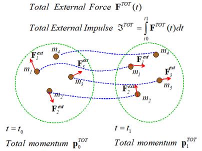
4.2.5 Impulse-momentum relation for a system of
particles
Suppose
we are interested in calculating the motion of several particles, sketched in
the figure.
Total external impulse on a system of
particles: Each particle in the
system can experience forces applied by:
Other particles in the system (e.g. due
to gravity, electric charges on the particles, or because the particles are
physically connected through springs, or because the particles collide). We call these internal forces acting in
the system. We will denote the internal
force exerted by the ith particle on
the jth particle by . Note that, because every action has an equal
and opposite reaction, the force exerted on the jth particle by the ith
particle must be equal and opposite, to ,
i.e. .
Forces exerted on the particles by the
outside world (e.g. by externally applied gravitational or
electromagnetic fields, or because the particles are connected to the outside
world through mechanical linkages or springs).
We call these external forces acting on the
system, and we will denote the external force on the i th particle by
We
define the total impulse exerted on
the system during a time interval as the sum of all the impulses on all the
particles. It’s easy to see that the
total impulse due to the internal forces is zero because the ith and jth particles
must exert equal and opposite impulses on one another, and when you add them up
they cancel out. So the total impulse on the system is simply
Total linear momentum of a system of particles: The total linear momentum of a system of particles is
simply the sum of the momenta of all the particles, i.e.
The
impulse-momentum equation
1. In differential form
2.
In integral form
This
is the integral of Newton’s
law of motion with respect to time.
Conservation of momentum: If no
external forces act on a system of particles, their total linear momentum is conserved, i.e.
Deriving the impulse-momentum equation
We start with the
impulse-momentum relation for a single particle in differential form
(The left hand side is the
total force on the ith particle it includes the external force, as well as all
the forces exerted by all the other particles).
Now sum over all the
particles
Notice that since
(To see this just write out
the full sum every internal force on one particle is equal
and opposite to the force on another, so the total has to cancel)
Therefore, evaluating the
sums
We can integrate this
expression with respect to time to get the integral version of the theorem.
4.2.6 Examples of applications of momentum
conservation for systems of particles
The
impulse-momentum equations for systems of particles are particularly useful for
(i) analyzing the recoil of a gun; and (ii) analyzing rocket and jet propulsion
systems. In both these applications, the
internal forces acting between the gun on the projectile, or the motor and
propellant, are much larger than any external forces, so the total momentum of
the system is conserved.
Example 1: Estimate the recoil velocity of a rifle (youtube
abounds with recoil demonstrations see. e.g. http://www.youtube.com/watch?v=F4juEIK_zRM
for samples. Be warned, however a lot of the videos are tasteless and/or
sexist… )
The
recoil velocity can be estimated by noting that the total momentum of bullet
and rifle together must be conserved. If
we can estimate the mass of rifle and bullet, and the bullet’s velocity, the
recoil velocity can be computed from the momentum conservation equation.
Assumptions:
1.
The mass of a
typical 0.22 (i.e. 0.22” diameter) caliber rifle bullet is about kg (idealizing the bullet as a sphere, with
density 7860 )
2.
The muzzle
velocity of a 0.22 is about 1000 ft/sec (305 m/s)
3.
A typical rifle
weighs between 5 and 10 lb (2.5-5 kg)
Calculation:
1.
Let denote the bullet mass, and let denote the mass of the rifle.
2.
The rifle and
bullet are idealized as two particles.
Before firing, both are at rest.
After firing, the bullet has velocity ;
the rifle has velocity .
3.
External forces
acting on the system can be neglected, so
.
4.
Substituting
numbers gives |V| between 0.04 and
0.08 m/s (about 0.14 ft/sec)
Example
2: Derive a formula that can be
used to estimate the mass of a handgun required to keep its recoil within
acceptable limits.
The
preceding example shows that the firearm will recoil with a velocity that
depends on the ratio of the mass of the bullet to the firearm. The firearm must be brought to rest by the person
holding it.
Assumptions:
1. We will idealize a person’s hand holding the gun as a
spring, with stiffness k, fixed at
one end. The ‘end-point stiffness’ of a
human hand has been extensively studied see, e.g. Shadmehr et al J. Neuroscience, 13
(1) 45 (1993). Typical values of
stiffness during quasi-static deflections are of order 0.2 N/mm. During dynamic
loading stiffnesses are likely to be larger than this.
2.
We idealize the handgun
and bullet as particles, with mass and ,
respectively.
Calculation.
1.
The preceding
problem shows that the firearm will recoil with velocity
2. Energy conservation can be used to calculate the
recoil distance. We consider the firearm
and the hand holding it a system. At
time t=0 it has zero potential
energy; and has kinetic energy . At the end of the recoil, the gun is at rest,
and the spring is fully compressed the kinetic energy is zero, and potential
energy is .
Energy
conservation gives
3. The required mass follows as .
Example 3 Rocket propulsion equations. Rocket
motors and jet engines exploit the momentum conservation law in order to
produce motion. They work by expelling
mass from a vehicle at very high velocity, in a direction opposite to the
motion of the vehicle. The momentum of
the expelled mass must be balanced by an equal and opposite change in the
momentum of the vehicle; so the velocity of the vehicle increases.
Analyzing
a rocket engine is quite complicated, because the propellant carried by the
engine is usually a very significant
fraction of the total mass of the vehicle.
Consequently, it is important to account for the fact that the mass
decreases as the propellant is used.
Assumptions:
1. The figure shows a rocket motor attached to a rocket
with mass M.
2. The rocket motor contains an initial mass of propellant and expels propellant at rate (kg/sec) with a velocity relative to the rocket.
3. We assume straight line motion, and assume that no
external forces act on the rocket or motor.
 Calculations:
The figure shows the rocket
at an instant of time t, and then a
very short time interval dt later.
1. At time t,
the rocket moves at speed v, and the system
has momentum ,
where m is the motor’s mass.
2. During the time
interval dt a mass is expelled
from the motor. The velocity of the expelled mass is .
3. At
time t+dt the mass of the motor has
decreased to .
4.
At time t+dt, the rocket has velocity .
5.
The total
momentum of the system at time t+dt is
therefore
6.
Momentum must be
conserved, so
7.
Multiplying this
out and simplifying shows that
where
the term has been neglected.
8.
Finally, we see
that
This result is called the
`rocket equation.’
Specific
Impulse of a rocket motor: The
performance of a rocket engine is usually specified by its `specific impulse.’ Confusingly, two different definitions of
specific impulse are commonly used:
The
first definition quantifies the impulse exerted by the motor per unit mass of
propellant; the second is the impulse per unit weight of propellant. You can usually tell which definition is
being used from the units the first definition has units of m/s; the
second has units of s. In terms of the
specific impulse, the rocket equation is
Integrated
form of the rocket equation: If the motor
expels propellant at constant rate, the equation of motion can be
integrated. Assume that
1.
The rocket is at
the origin at time t=0;
2.
The rocket has
speed at time t=0
3.
The motor has mass at time t=0;
this means that at time t it has mass
Then the rocket’s speed can be calculated as a function of
time:
Similarly, the position
follows as
These
calculations assume that no external forces act on the rocket. It is quite straightforward to generalize
them to account for external forces as well the details are left as an exercise.
Example 4 Application of rocket
propulsion equation: Calculate the maximum
payload that can be launched to escape velocity on the Ares I launch vehicle.
‘Escape velocity’ means that after the motor burns out, the space
vehicle can escape the earth’s gravitational field see example 5 in Section 4.1.6.
Assumptions
1. The specifications for the Ares I are at http://www.braeunig.us/space/specs/ares.htm
Relevant variables are listed in the
table below.
|
|
Total
mass (kg)
|
Specific
impulse (s)
|
Propellant
mass (kg)
|
|
Stage
I
|
586344
|
268.8
|
504516
|
|
Stage
II
|
183952
|
452.1
|
163530
|
2.
As an
approximation, we will neglect the motion of the rocket during the burn, and will
neglect aerodynamic forces.
3.
We will assume
that the first stage is jettisoned before burning the second stage.
4.
Note that the
change in velocity due to burning a stage can be expressed as
where is the total mass before the burn, and is the mass of propellant burned.
- The earth’s radius is 6378.145km
- The Gravitational parameter (G=
gravitational constant; M=mass
of earth)
- Escape velocity is from the earths surface is ,
where R
is the earth’s radius.
Calculation:
1. Let m denote
the payload mass; let denote the total masses of stages I and II,
let denote the propellant masses of stages I and
II; and let ,
denote the specific impulses of the two
stages.
2. The rocket is at rest before burning the first stage;
and its total mass is . After burn, the mass is . The velocity after burning the first stage is
therefore
3. The first stage is then jettisoned the mass before starting the second burn is ,
and after the second burn it is . The velocity after the second burn is
therefore
4. Substituting numbers into the escape velocity formula
gives km/sec.
Substituting numbers for the masses shows that to reach this velocity,
the payload mass must satisfy
where m is
in kg.
5. We can use Matlab to solve for the critical value of m for equality
clear
all
syms
m
eq
=
11.1798==2.62908*log((m+770296)/(m+265780))+4.435101*log((m+183952)/(m+20422))
solve(eq,m)

so
the solution is 8300kg a very small mass compared with that of the
launch vehicle, but you could pack in a large number of people you would like
to launch into outer space nonetheless (the entire faculty of the school of
engineering, if you wish).
4.2.7 Analyzing collisions between particles: the
restitution coefficient
The
momentum conservation equations are particularly helpful if you want to analyze
collisions between two or more objects. If
the impact occurs over a very short time, the impulse exerted by the contact
forces acting at the point of collision is huge compared with the impulse
exerted by any other forces. If we
consider the two colliding particles as a system, the external impulse exerted
on the system can be taken to be zero, and so the total momentum of the system
is conserved.
The
momentum conservation equation can be used to relate the velocities of the
particles before collision to those after collision. These relations are not enough to be able to
determine the velocities completely, however to do this, we also need to be able to
quantify the energy lost (or more accurately, dissipated as heat) during the
collision.
In
practice we don’t directly specify the energy loss during a collision instead, the relative velocities are related
by a property of the impact called the coefficient
of restitution.
Restitution
coefficient for straight line motion
Suppose that two colliding
particles A and B move in a straight line parallel to a unit vector i. Let
denote the velocities of A and B just before
the collision
denote the velocities of A and B just after
the collision.
The velocities before and
after impact are related by
where
e is the restitution coefficient. The
negative sign is needed because the particles approach one another before
impact, and separate afterwards.
Restitution
coefficient for 3D frictionless collisions
For a more general contact,
we define
to denote velocities of the particles before
collision
to denote velocities of the particles after
collision
In
addition, we let n be a unit vector
normal to the common tangent plane at the point of contact (if the two
colliding particles are spheres or disks the vector is parallel to the line
joining their centers).
The velocities before and
after impact are related by two vector equations:
To interpret these
equations, note that
1. The first equation states that the component of
relative velocity normal to the contact plane is reduced by a factor e (just as for 1D contacts)
2. The second equation states that the component of
relative velocity tangent to the contact plane is unchanged
To
understand the second equation, note that.
·
During the
collision, a very large force acts on both A and B at the contact between
them. Because the contact is
frictionless, the direction of the force must be parallel to n.
Also, the force on A must be equal and opposite to the force on B.
·
There is no force
acting on either A or B parallel to t. This means that momentum must be conserved
in the t direction for both A and B
individually. We can write this
mathematically as
(this looks funny, but we have just subtracted the
normal component of velocity from the total velocity. This leaves just the tangential
component). Subtracting the second
equation from the first shows that
Combined 3D restitution formula
The
two equations for the normal and tangential behavior can be combined (just add
them) into a single vector equation relating velocities before and after impact
this form is more compact, and often more
useful, but more difficult to visualize physically
Values of
restitution coefficient
The
restitution coefficient almost always lies in the range . It can only be less than zero if one object
can penetrate and pass through the other (e.g. a bullet); and can only be
greater than 1 if the collision generates energy somehow (e.g. releasing a
preloaded spring, or causing an explosion).
If
e=0, the two colliding objects stick
together; if e=1 the collision is
perfectly elastic, with no energy loss.
The
restitution coefficient is strongly sensitive to the material properties of the
two colliding objects, and also varies weakly with their geometry and the
velocity of impact. The two latter
effects are usually ignored.
Collision
between a particle and a fixed rigid surface. The collision formulas can be applied to impact between a rigid fixed
surface by taking the surface to be particle B, and noting that the velocity of particle B is then zero both before and after impact.
For straight line motion,
For
collision with an angled wall ,
where
n is a unit
vector perpendicular to the wall.
4.2.8 Examples of collision problems
Example 1 Suppose that a moving car hits a stationary (parked)
vehicle from behind. Derive a formula
that will enable an accident investigator to determine the velocity of the
moving car from the length of the skid marks left on the road.
Assumptions:
1.
We will assume
both cars move in a straight line
2.
The moving and
stationary cars will be assumed to have masses ,
respectively
3.
We will assume
the cars stick together after the collision (i.e. the restitution coefficient
is zero)
4.
We will assume
that only the parked car has brakes applied after the collision
This
calculation takes two steps: first, we will use work-energy to relate the
distance slid by the cars after impact to their velocity just after the impact
occurs. Then, we will use momentum and the restitution formula to work out the
velocity of the moving car just before impact.
Calculation:
Let V denote the velocity of the moving car just before impact; let denote the velocity of the two (connected)
cars just after impact, and let d denote
the distance slid.
1. The figure shows a free body diagram for each of the
two cars during sliding after the collision.
Newton’s
law of motion for each car shows that
2.
The vertical
component of the equations of motion give ;
.
3. The parked car has locked wheels and skids over the
road; the friction law gives the tangential forces at the contacts as
4. We can calculate the velocity of the cars just after
impact using the work-kinetic energy relation during skidding. For this purpose, we consider the two
connected cars as a single particle. The
work done on the particle by the friction forces is . The work done is equal to the change in
kinetic energy of the particle, so
5. Finally, we can use momentum conservation to calculate
the velocity just before impact. The
momentum after impact is ,
while before impact . Equating the two gives
Example 2: Two frictionless spheres with radius R have initial velocity . At some instant of time, the two particles
collide. At the point of collision, the centers
of the spheres have position vectors . The restitution coefficient for the contact
is denoted by e. Find a formula for
the velocities of the spheres after impact.
Hence, deduce an expression for the change in kinetic energy during the
impact.
This is a straightforward vector algebra
exercise. We have two unknown velocity
vectors: ,
and two vector equations momentum conservation, and the restitution
coefficient formula.
Calculation
1. Note that a unit vector normal to the tangent plane
can be calculated from the position vectors of the centers at the impact as . It doesn’t matter whether you choose to take n to point from A to B or the other way
around the formula will work either way.
2.
Momentum
conservation requires that
3.
The restitution
coefficient formula gives
4. We can solve (2) and (3) for by multiplying (3) by and adding the equations, which gives
5. Similarly, we can solve for by multiplying (3) by and subtracting (3) from (2), with the result
6. The change in kinetic energy during the collision can
be calculated as
7.
Substituting the
results of (4) and (5) for and and simplifying the result gives
Note
that the energy change is zero if e=1
(perfectly elastic collisions) and is always negative for e<1 (i.e. the kinetic energy after collision is less than that
before collision).
 Example 3: This is just a boring example to help illustrate the
practical application of the vector formulas in the preceding example. In the figure shown, disk A has a vertical velocity V at time t=0, while disk B is stationary.
The two disks both have radius R,
have the same mass, and the restitution coefficient between them is e. Gravity can be neglected. Calculate
the velocity vector of each disk after collision.
Example 3: This is just a boring example to help illustrate the
practical application of the vector formulas in the preceding example. In the figure shown, disk A has a vertical velocity V at time t=0, while disk B is stationary.
The two disks both have radius R,
have the same mass, and the restitution coefficient between them is e. Gravity can be neglected. Calculate
the velocity vector of each disk after collision.
Calculation
1. Before impact, the velocity vectors are
2. A unit vector parallel to the line joining the two
centers is (to see this, apply Pythagoras theorem to the
triangle shown in the figure).
3. The velocities after impact are
Substituting the vectors gives
 Example 4: How to play pool (or snooker, billiards, or your own
favorite bar game involving balls, a stick, and a table…). The figure shows a typical problem faced by a
pool player where should the queue ball hit the eight ball
to send it into the pocket?
Example 4: How to play pool (or snooker, billiards, or your own
favorite bar game involving balls, a stick, and a table…). The figure shows a typical problem faced by a
pool player where should the queue ball hit the eight ball
to send it into the pocket?
This
is easily solved the eight ball is stationary before impact,
and after impact has a velocity
Notice
that the velocity is parallel to the unit vector n. This vector is parallel
to a line connecting the centers of the two balls at the instant of impact. So
the correct thing to do is to visualize an imaginary ball just touching the
eight ball, in line with the pocket, and aim the queue ball at the imaginary
ball. Easy!
 The real secret to being a successful pool player is
not potting the balls that part is easy. It is controlling where the queue ball goes
after impact. You may have seen experts
make a queue ball reverse its direction after an impact (appearing to bounce
off the stationary ball); or make the queue ball follow the struck ball after
the impact. According to the simple equations
developed here, this is impossible but a pool table is more complicated, because
the balls rotate, and are in contact with a table. By giving the queue ball spin, an expert player can move the queue ball around at will. To make the ball rebound, it must be struck
low down (below the ‘center of percussion’) to give it a reverse spin; to make
it follow the struck ball, it should be struck high up, to make it roll towards
the ball to be potted. Giving the ball
a sideways spin can make it rebound in a controllable direction laterally as
well. And it is even possible to make a
queue ball travel in a curved path
with the right spin.
The real secret to being a successful pool player is
not potting the balls that part is easy. It is controlling where the queue ball goes
after impact. You may have seen experts
make a queue ball reverse its direction after an impact (appearing to bounce
off the stationary ball); or make the queue ball follow the struck ball after
the impact. According to the simple equations
developed here, this is impossible but a pool table is more complicated, because
the balls rotate, and are in contact with a table. By giving the queue ball spin, an expert player can move the queue ball around at will. To make the ball rebound, it must be struck
low down (below the ‘center of percussion’) to give it a reverse spin; to make
it follow the struck ball, it should be struck high up, to make it roll towards
the ball to be potted. Giving the ball
a sideways spin can make it rebound in a controllable direction laterally as
well. And it is even possible to make a
queue ball travel in a curved path
with the right spin.
Never
let it be said that you don’t learn useful skills in engineering classes!
4.3 Angular impulse-momentum relations
4.3.1 Definition of the angular impulse
of a force
The angular impulse of a
force is the time integral of the moment
exerted by the force.
To make the concept precise, consider a particle that
is subjected to a time varying force ,
with components in a fixed basis ,
then
Let
denote the position vector
of the particle, and
the moment of the force
about the origin.
The Angular Impulse exerted
by the force about O during a time interval is defined as
The angular impulse is a
vector, and can be expressed as components in a basis
If you know the moment as a
function of time, you can calculate its angular impulse using simple
calculus. For example for a constant moment, with vector value ,
the impulse is
4.3.2 Definition of the angular momentum of a particle
The angular momentum of a
particle is simply the cross product of the particle’s position vector with its
linear momentum
The
angular momentum is a vector the direction of the vector is perpendicular
to its velocity and its position vectors.
4.3.3 Angular impulse Angular Momentum relation for a single
particle
Consider a particle that is subjected to a
force for a time interval .
Let denote the position vector of the particle
Let denote the moment of F about the origin
Let A
denote the angular impulse exerted on the particle
Let denote the angular momentum at time
Let denote the angular momentum at time
The
momentum conservation equation can be expressed either in differential or
integral form.
1.
In differential
form
2.
In integral form
Proof: Although it’s not obvious, these are just another way
of writing Newton’s laws of motion. To
show this, we’ll derive the differential form.
Start with Newton’s
law
Take the cross product of
both sides with r
Note
that since the cross product of two parallel
vectors is zero. We can add this to the
right hand side, which shows that
This yields the required
relation.
Angular
momentum conservation: For the
special case where the force is parallel
to r, the moment of the force acting
on the particle is zero ( ), and angular momentum is constant
4.3.4 Examples using Angular Impulse Angular Momentum relations for a single
particle
The
angular impulse-angular momentum equations are particularly helpful when you
need to solve problems where particles are subjected to a single force, which
acts through a fixed point. They can also be used to analyze rotational motion
of a massless frame containing one or more particles.
Example
1: Orbital motion. A satellite is launched into a geostationary
transfer orbit by the ARIANE V launch facility.
At its perigee (the point where the satellite is closest to the earth)
the satellite has speed 10.2km/sec and altitude 250km. At apogee (the point where the satellite is
furthest from the earth) the satellite has altitude 35950 km. Calculate the speed of the satellite at
apogee.
Assumptions:
1.
We assume that
the only force acting on the satellite is the gravitational attraction of the
earth
2.
The earth’s
radius is 6378.145km
Calculation:
1. Since the gravitational force on the satellite always
acts towards the center of the earth, angular momentum about the earth’s center
is conserved.
2. At both perigee and apogee, the velocity vector of the
satellite must be perpendicular to its position vector. To see this, note that
at the point where the satellite is closest and furthest from the earth, the
distance to the earth is a max or min, and so the derivative of the distance of
the satellite from the earth must vanish, i.e.
where
we have used the chain rule to evaluate the time derivative of . Recall that
if the dot product of two vectors vanishes, they are mutually perpendicular. We
take a coordinate system with i and j in the plane of the orbit, and k perpendicular to the orbit.
3.
We take the
satellite orbit to lie in the i , j plane with k perpendicular to the orbit.
The angular momentum at apogee and perigee is then
where are the distance of the satellite from the
center of the earth at apogee and perigee, and are the corresponding speeds.
4. Since angular momentum is conserved it follows that
5.
Substituting
numbers yields 1.6 km/s
 Example 2: More orbital motion. The orbit for a satellite is normally specified by a
set of angles specifying the inclination of the orbit, and by quoting the
distance of the satellite from the earths center at apogee and perigee . It is possible to calculate the speed of the
satellite at perigee and apogee from this information.
Example 2: More orbital motion. The orbit for a satellite is normally specified by a
set of angles specifying the inclination of the orbit, and by quoting the
distance of the satellite from the earths center at apogee and perigee . It is possible to calculate the speed of the
satellite at perigee and apogee from this information.
Calculation
1. From the previous example, we know that the distances
and velocities are related by
2.
The system is
conservative, so the total energy of the system is conserved.
3.
The potential energies
when the satellite is at perigee and apogee are
4.
The kinetic
energies of the satellite at perigee and apogee are
5.
The kinetic
energy of the earth can be assumed to be constant. Energy conservation therefore shows that
6.
The results of
(1) and (5) give two equations that can be solved for in terms of known parameters. For example, (1) shows that - this can be substituted into (5) to see that
Similarly,
at apogee
4.4 Summary of definitions and equations
Work, Power, Kinetic Energy
The Power
developed by a force, (or the rate of
work done by the force) is
.
The work
done by the force during a time
interval is
The work done by the force
can also be calculated by integrating the force vector along the path traveled
by the force, as
where are the initial and final positions of the
force.
The Kinetic
Energy of a particle is
Conservative forces and potential energy
A
force (or pair of forces) is conservative
if the work done by the force when it moves between any two points is the same
for all paths joining the two points
The
potential
energy of a conservative force is defined as the negative of the work
done by the force in moving from some arbitrary initial position to a new position ,
i.e.
Alternatively
Table
of potential energy relations
In
practice, however, we rarely need to do the integrals to calculate the
potential energy of a force, because there are very few different kinds of
force. For most engineering calculations
the potential energy formulas listed in the table below are sufficient.
|
Type of force
|
Force vector
|
Potential energy
|
|
|
Gravity acting on a particle near earths surface
|
|
|
|
|
Gravitational force exerted on mass m by mass M at the
origin
|
|
|
|
|
Force exerted by a spring with stiffness k and unstretched length
|
|
|
|
|
Force acting between two charged particles
|
|
|
|
|
Force exerted by one molecule of a noble gas (e.g. He, Ar,
etc) on another (Lennard Jones potential). a is the equilibrium spacing between molecules, and E is the energy of the bond.
|
|
|
|
Power-Work-kinetic energy relations for
a single particle
The
Power-kinetic energy relation for the
particle states that the rate of work done by F is equal to the rate of change of kinetic energy of the particle,
i.e.
|
|
|
|
The
Work-kinetic energy relation for a
particle says that the total work done by the force F on the particle is equal to the change in the kinetic energy of
the particle.
Power-Work-kinetic energy relations for
a conservative system of particles
A
system is conservative if a potential energy can be defined for all internal
forces in the system
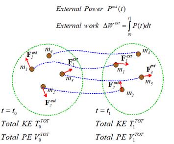
- At some time the system has and kinetic energy
- At some later time the system has kinetic energy .
- Let denote the potential energy of the
internal forces at time
- Let denote the potential energy of the internal
forces at time
- Let denote the total work done on the system
between
Power Energy Relation:
Work Energy Relation:
Energy
conservation law
Linear impulse of a force
Linear momentum of a particle
The linear momentum of a
particle is simply the product of its mass and velocity
The linear momentum is a
vector its direction is parallel to the velocity of the
particle.
Impulse-momentum relations for a single particle
Consider a particle that is subjected to a
force for a time interval .
Let denote the impulse exerted by F on the particle
Let denote the linear momentum of the particle at
time .
Let denote the linear momentum of the particle at
time .
In
differential form
In
integral form
This
is the integral of Newton’s
law of motion with respect to time.
Impulse-momentum relations for a system of particles
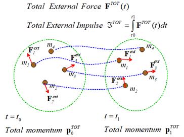
In differential form
In
integral form
If no
external forces act on a system of particles, their total linear momentum is conserved, i.e.
Collisions
If no external impulse acts
on two particles as they collide, their total momentum is conserved.
To calculate velocities
after impact we define the restitution
coefficient
Restitution
coefficient for straight line motion
denote the velocities of A and B just before
the collision
denote the velocities of A and B just after
the collision.
The velocities before and
after impact are related by
where
e is the restitution coefficient.
Restitution
coefficient for 3D frictionless collisions
Define
to denote velocities of the particles before
collision
to denote velocities of the particles after
collision
In
addition, we let n be a unit vector
normal to the common tangent plane at the point of contact (if the two
colliding particles are spheres or disks the vector is parallel to the line
joining their centers).
The velocities before and
after collision are related by
Angular
impulse
The Angular Impulse exerted
by the force about O during a time interval is defined as
Angular momentum of a particle
Angular impulse Angular Momentum relation for a single
particle
Consider a particle that is subjected to a
force for a time interval .
Let denote the position vector of the particle
Let denote the moment of F about the origin
Let A
denote the angular impulse exerted on the particle
Let denote the angular momentum at time
Let denote the angular momentum at time
In
differential form
In
integral form

 Example 1: The longest single-span escalator in the Western
hemisphere is located at the Washington Metro station in Montgomery County,
Maryland. Some technical specifications
for the escalator span can be found on Wikipedia (we
have not checked this data!).
Additional information concerning escalator standards can be found here.
Example 1: The longest single-span escalator in the Western
hemisphere is located at the Washington Metro station in Montgomery County,
Maryland. Some technical specifications
for the escalator span can be found on Wikipedia (we
have not checked this data!).
Additional information concerning escalator standards can be found here.