Chapter 2
Review of Forces and Moments
2.1 Forces
In
this chapter we review the basic concepts of forces, and force laws. Most of this material is identical to
material covered in EN030, and is provided here as a review. There are a few
additional sections for example forces exerted by a damper or dashpot, an inerter, and interatomic forces are discussed in
Section 2.1.7.
2.1.1 Definition of a force
Engineering
design calculations nearly always use classical (Newtonian) mechanics. In
classical mechanics, the concept of a `force’ is based on experimental
observations that everything in the universe seems to have a preferred
configuration masses appear to attract each other; objects
with opposite charges attract one another; magnets can repel or attract one
another; you are probably repelled by your professor. But we don’t really know why this is
(except perhaps the last one).
The
idea of a force is introduced to quantify the tendency of objects to
move towards their preferred configuration.
If objects accelerate very quickly towards their preferred
configuration, then we say that there’s a big force acting on them. If they
don’t move (or move at constant velocity), then there is no force. We can’t see
a force; we can only deduce its existence by observing its effect.
Specifically, forces are
defined through Newton’s
laws of motion
 0. A `particle’ is a small mass at some position in space.
1.
When the sum of the forces acting on a particle is zero, its velocity is
constant;
2.
The sum of forces acting on a particle of constant mass is equal to the product
of the mass of the particle and its acceleration;
3.
The forces exerted by two particles on each other are equal in magnitude and
opposite in direction.
Isaac Newton on a bad hair day
The second law provides the
definition of a force if a mass m has acceleration a,
the force F acting on it is
Of course, there is a big
problem with Newton’s
laws what do we take as a fixed point (and
orientation) in order to define acceleration?
The general theory of relativity addresses this issue rigorously. But for engineering calculations we can
usually take the earth to be fixed, and happily apply Newton’s laws. In rare cases where the earth’s motion is
important, we take the stars far from the solar system to be fixed.
2.1.2 Causes of force
Forces may arise from a
number of different effects, including
(i)
Gravity;
(ii)
Electromagnetism or electrostatics;
(iii)
Pressure exerted by fluid or gas on part of a structure
(v)
Wind or fluid induced drag or lift forces;
(vi)
Contact forces, which act wherever a structure or component touches anything;
(vii)
Friction forces, which also act at contacts.
Some
of these forces can be described by universal laws. For example, gravity forces can be calculated
using Newton’s
law of gravitation; electrostatic forces acting between charged particles are
governed by Coulomb’s law; electromagnetic forces acting between current
carrying wires are governed by Ampere’s law; buoyancy forces are governed by
laws describing hydrostatic forces in fluids. Some of these universal force laws are listed
in Section 2.6.
Some
forces have to be measured. For example, to determine friction forces acting in
a machine, you may need to measure the coefficient of friction for the
contacting surfaces. Similarly, to
determine aerodynamic lift or drag forces acting on a structure, you would
probably need to measure its lift and drag coefficient experimentally. Lift and drag forces are described in Section
2.6. Friction forces are discussed in
Section 12.
Contact
forces are pressures that act on the
small area of contact between two objects.
Contact forces can either be measured, or they can be calculated by
analyzing forces and deformation in the system of interest. Contact forces are very complicated, and are
discussed in more detail in Section 8.
2.1.3 Units of force and
typical magnitudes
In SI units, the
standard unit of force is the Newton,
given the symbol N.
The Newton is a derived unit, defined
through Newton’s
second law of motion a force of 1N causes a 1 kg mass to accelerate
at 1 .
The fundamental unit of
force in the SI convention is kg m/s2
In US units, the
standard unit of force is the pound, given the symbol lb or lbf (the latter is
an abbreviation for pound force, to distinguish it from pounds weight)
A force of 1 lbf causes a
mass of 1 slug to accelerate at 1 ft/s2
US
units have a frightfully confusing way of representing mass often the mass of an object is reported as weight,
in lb or lbm (the latter is an abbreviation for pound mass). The weight of an object in lb is not mass at
all it’s actually the gravitational force acting on the mass. Therefore, the mass of an object in slugs
must be computed from its weight in pounds using the formula
where g=32.1740 ft/s2
is the acceleration due to gravity.
A force of 1 lb(f) causes a
mass of 1 lb(m) to accelerate at 32.1740 ft/s2
The conversion factors from
lb to N are
|
1 lb
|
=
|
4.448 N
|
|
1 N
|
=
|
0.2248 lb
|
(www.onlineconversion.com is a handy
resource, as long as you can tolerate all the hideous advertisements…)
As
a rough guide, a force of 1N is about equal to the weight of a medium sized
apple. A few typical force magnitudes (from `The Sizesaurus’, by Stephen
Strauss, Avon Books, NY, 1997) are listed in the table below
|
Force
|
Newtons
|
Pounds Force
|
|
Gravitational Pull of the
Sun on Earth
|
|
|
|
Gravitational Pull of the
Earth on the Moon
|
|
|
|
Thrust of a Saturn V
rocket engine
|
|
|
|
Thrust of a large jet
engine
|
|
|
|
Pull of a large
locomotive
|
|
|
|
Force between two protons
in a nucleus
|
|
|
|
Gravitational pull of the
earth on a person
|
|
|
|
Maximum force exerted
upwards by a forearm
|
|
|
|
Gravitational pull of the
earth on a 5 cent coin
|
|
|
|
Force between an electron
and the nucleus of a Hydrogen atom
|
|
|
2.1.4 Classification of
forces: External forces, constraint forces and internal forces.
When analyzing forces in a
structure or machine, it is conventional to classify forces as external
forces; constraint forces or internal forces.
External forces arise from interaction between the system of interest
and its surroundings.
Examples
of external forces include gravitational forces; lift or drag forces arising
from wind loading; electrostatic and electromagnetic forces; and buoyancy
forces; among others. Force laws
governing these effects are listed later in this section.
Constraint forces are exerted by one part of a structure on another, through joints,
connections or contacts between components.
Constraint forces are very complex, and will be discussed in detail in
Section 8.
Internal
forces are forces that act inside a
solid part of a structure or component.
For example, a stretched rope has a tension
force acting inside it, holding the rope together. Most solid objects contain very complex
distributions of internal force. These
internal forces ultimately lead to structural failure, and also cause the
structure to deform. The purpose of
calculating forces in a structure or component is usually to deduce the
internal forces, so as to be able to design stiff, lightweight and strong
components. We will not, unfortunately,
be able to develop a full theory of internal forces in this course a proper discussion requires understanding of
partial differential equations, as well as vector and tensor calculus. However, a brief discussion of internal
forces in slender members will be
provided in Section 9.
2.1.5 Mathematical
representation of a force.
Force is a vector it has a magnitude (specified in Newtons, or lbf, or
whatever), and a direction.
A force is therefore always
expressed mathematically as a vector quantity.
To do so, we follow the usual rules, which are described in more detail
in the vector tutorial. The procedure is
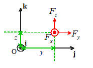
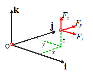
1.
Choose basis
vectors or that establish three fixed (and usually
perpendicular) directions in space;
2.
Using geometry or
trigonometry, calculate the force component along each of the three reference
directions or ;
3.
The vector force
is then reported as
For calculations, you will
also need to specify the point where the force acts on your system or
structure. To do this, you need to
report the position vector of the point where the force acts on the
structure.
The procedure for
representing a position vector is also described in detail in the vector
tutorial. To do so, you need to:
1.
Choose an origin
2.
Choose basis
vectors or that establish three fixed directions in space
(usually we use the same basis for both force and position vectors)
3.
Specify the
distance you need to travel along each direction to get from the origin to the
point of application of the force or
4.
The position
vector is then reported as
2.1.6 Measuring forces
Engineers
often need to measure forces. According to the definition, if we want to
measure a force, we need to get hold of a 1 kg mass, have the force act on it
somehow, and then measure the acceleration of the mass. The magnitude of the
acceleration tells us the magnitude of the force; the direction of motion of
the mass tells us the direction of the force.
Fortunately, there are easier ways to measure forces.
In addition to causing acceleration, forces
cause objects to deform for example, a force will stretch or compress
a spring; or bend a beam. The
deformation can be measured, and the force can be deduced.
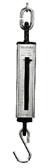
The
simplest application of this phenomenon is a spring scale. The change in length of a spring is proportional
to the magnitude of the force causing it to stretch (so long as the force is
not too large!) this
relationship is known as Hooke’s law and can be expressed as an equation
where the spring stiffness depends on the material the spring is made
from, and the shape of the spring. The
spring stiffness can be measured experimentally to calibrate the spring.
Spring
scales are not exactly precision instruments, of course. But the same principle is used in more
sophisticated instruments too. Forces
can be measured precisely using a `force transducer’ or `load cell’ (A search
for `force transducer’ on any search engine will bring up a huge variety of
these a few are shown in the picture). The simplest load cell works much like a
spring scale you can load it in one direction, and it will
provide an electrical signal proportional to the magnitude of the force. Sophisticated load cells can measure a force vector,
and will record all three force components.
Really fancy load cells measure both force vectors, and torque or moment
vectors.

Simple force transducers capable of measuring a single
force component. The instrument on the
right is called a `proving ring’ there’s a short article describing how it
works at http://www.mel.nist.gov/div822/proving_ring.htm
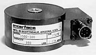
A sophisticated force transducer produced by MTS
systems, which is capable of measuring forces and moments acting on a car’s
wheel in-situ. The spec for this
device can be downloaded at http://www.mts.com/cs/groups/public/documents/library/dev_002232.pdf
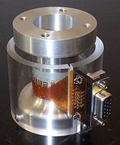
The basic design of all
these load cells is the same they measure (very precisely) the deformation
in a part of the cell that acts like a very stiff spring. One example (from Sandia National Lab
) is shown on the right. In this case
the `spring’ is actually a tubular piece of high-strength steel. When a force acts on the cylinder, its length
decreases slightly. The deformation is
detected using `strain gages’ attached to the cylinder. A strain gage is really
just a thin piece of wire, which deforms with the cylinder. When the wire gets shorter, its electrical
resistance decreases this resistance change can be measured, and
can be used to work out the force. It is
possible to derive a formula relating the force to the change in resistance,
the load cell geometry, and the material properties of steel, but the
calculations involved are well beyond the scope of this course.
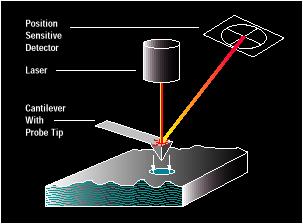 The most sensitive load cell currently available is
the atomic force microscope (AFM) which as the name suggests, is intended to
measure forces between small numbers of atoms.
This device consists of a very thin (about 1 ) cantilever beam, clamped at one end, with a
sharp tip mounted at the other. When the
tip is brought near a sample, atomic interactions exert a force on the tip and
cause the cantilever to bend. The
bending is detected by a laser-mirror system.
The device is capable of measuring forces of about 1 pN (that’s N!!), and is used to explore the properties of
surfaces, and biological materials such as DNA strands and cell membranes. A nice article on the AFM can be found at http://www.di.com
The most sensitive load cell currently available is
the atomic force microscope (AFM) which as the name suggests, is intended to
measure forces between small numbers of atoms.
This device consists of a very thin (about 1 ) cantilever beam, clamped at one end, with a
sharp tip mounted at the other. When the
tip is brought near a sample, atomic interactions exert a force on the tip and
cause the cantilever to bend. The
bending is detected by a laser-mirror system.
The device is capable of measuring forces of about 1 pN (that’s N!!), and is used to explore the properties of
surfaces, and biological materials such as DNA strands and cell membranes. A nice article on the AFM can be found at http://www.di.com
Selecting a load cell
As an engineer, you may
need to purchase a load cell to measure a force. Here are a few considerations that will guide
your purchase.
1.
How many force
(and maybe moment) components do you need to measure? Instruments that measure several force
components are more expensive…
2.
Load capacity what is the maximum force you need to measure?
3.
Load range what is the minimum force you need to measure?
4.
Accuracy
5.
Temperature
stability how much will the reading on the cell change
if the temperature changes?
6.
Creep stability if a load is applied to the cell for a long
time, does the reading drift?
7.
Frequency
response how rapidly will the cell respond to time
varying loads? What is the maximum
frequency of loading that can be measured?
8.
Reliability
9.
Cost
2.1.7 Force Laws
In this section, we list
equations that can be used to calculate forces associated with
(i)
Gravity
(ii)
Forces exerted by
linear springs
(iii)
Electrostatic
forces
(iv)
Electromagnetic
forces
(v)
Hydrostatic
forces and buoyancy
(vi)
Aero- and hydro-dynamic
lift and drag forces
Gravitation
Gravity forces acting on
masses that are a large distance apart
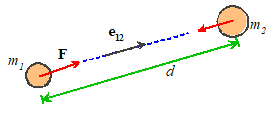
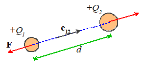
Consider
two masses and that are a distance d apart. Newton’s
law of gravitation states that mass will experience a force
where
is a unit vector pointing from mass to mass ,
and G is the Gravitation constant. Mass will experience a force of equal magnitude,
acting in the opposite direction.
In SI units,
The
law is strictly only valid if the masses are very small (infinitely small,
in fact) compared with d so the formula works best for calculating the
force exerted by one planet or another; or the force exerted by the earth on a
satellite.
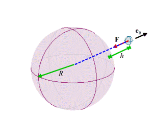 Gravity forces acting on a small object close to the
earth’s surface
Gravity forces acting on a small object close to the
earth’s surface
For engineering purposes,
we can usually assume that
1.
The earth is spherical,
with a radius R
2.
The object of
interest is small compared with R
3.
The object’s
height h above the earths surface is
small compared to R
If the first two
assumptions are valid, then one can show that Newton’s law of gravitation implies that a mass
m at a height h above the earth’s surface experiences a force
where
M is the mass of the earth; m
is the mass of the object; R is the earth’s radius, G is the
gravitation constant and is a unit vector pointing from the center of
the earth to the mass m. (Why do
we have to show this? Well, the mass m actually experiences a force of
attraction towards every point inside the earth. One might guess that points close to the
earth’s surface under the mass would attract the mass more than those far away,
so the earth would exert a larger gravitational force than a very small object
with the same mass located at the earth’s center. But this turns out not to be the case, as
long as the earth is perfectly uniform and spherical).
If the third assumption (h<<R) is valid, then we can
simplify the force law by setting
where g is a constant, and j is a `vertical’ unit vector (i.e.
perpendicular to the earth’s surface).
In SI units .
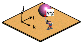
The
force of gravity acts at the center of gravity of an object. For most engineering calculations the center
of gravity of an object can be assumed to be the same as its center of
mass. For example, gravity would exert a
force at the center of the sphere that Mickey is holding. The location of the center of mass for
several other common shapes is shown below.
The procedure for calculating center of mass of a complex shaped object
is discussed in more detail in section 6.3.
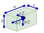
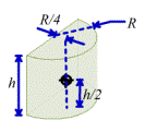
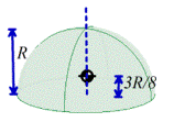
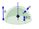
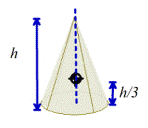
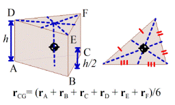
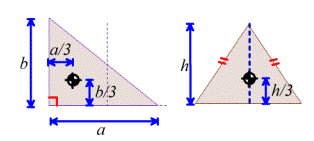
|
TABLE OF
POSITIONS OF CENTER OF MASS FOR COMMON OBJECTS
|
|
|
|
|
|
Rectangular prism
|
Circular cylinder
|
Half-cylinder
|
|
|
|
|
|
|
|
|
|
Solid hemisphere
|
Thin hemispherical shell
|
Cone
|
|
|
|
|
|
|
|
Triangular Prism
Thin triangular laminate
|
Some subtleties about
gravitational interactions
There
are some situations where the simple equations in the preceding section don’t
work. Surveyors know perfectly well that
the earth is no-where near spherical; its density is also not uniform. The earth’s gravitational field can be quite
severely distorted near large mountains, for example. So using the simple gravitational formulas in
surveying applications (e.g. to find the `vertical’ direction) can lead to
large errors.
Also,
the center of gravity of an object is not
the same as its center of mass. Gravity
is actually a distributed force. When
two nearby objects exert a gravitational force on each other, every point in
one body is attracted towards every point inside its neighbor. The distributed force can be replaced by a
single, statically equivalent force, but the point where the equivalent force
acts depends on the relative positions of the two objects, and is not generally
a fixed point in either solid. One
consequence of this behavior is that gravity can cause rotational
accelerations, as well as linear accelerations.
For example, the resultant force of gravity exerted on the earth by the
sun and moon does not act at the center of mass of the earth. As a result, the earth precesses that is to say, its axis of rotation changes
with time.
Forces exerted by springs
A
solid object (e.g. a rubber band) can be made to exert forces by stretching
it. The forces exerted by a solid that
is subjected to a given deformation depend on the shape of the component, the
materials it is made from, and how it is connected to its surroundings. Solid
objects can also exert moments, or torques we will define these shortly. Forces
exerted by solid components in a machine or structure are complicated, and will
be discussed in detail separately.
Here, we restrict attention to the simplest case: forces exerted by
linear springs.
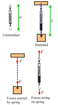
A spring scale is a good
example of a linear spring. You can
attach it to something at both ends. If you
stretch or compress the spring, it will exert forces on whatever you connected
to.
The forces exerted by the
ends of the spring always act along the line of the spring. The magnitude of the force is (so long as you
don’t stretch the spring too much) given by the formula
where a is the un-stretched spring length; L is the stretched length, and k
is the spring stiffness.
In the SI system, k has units of N/m.
Note that when you draw a
picture showing the forces exerted by a spring, you must always assume that the
spring is stretched, so that the forces exerted by the spring are attractive. If you don’t do this, your sign convention
will be inconsistent with the formula ,
which assumes that a compressed spring (L<a)
exerts a negative force.
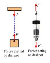
Forces exerted by dashpots
A
‘Dashpot’ is somewhat like a spring except that it exerts forces that are
proportional to the relative velocity of its two ends, instead of the relative
displacement. The device is extremely
useful for damping vibrations. The
device usually consists of a plunger that forces air or fluid through a small
orifice the force required to expel the fluid is
roughly proportional to the velocity of the plunger. For an example of a precision dashpot see http://www.airpot.com/beta/html/dashpot_defined.html
The forces exerted by the
ends of the dashpot always act along the line of the dashpot. The magnitude of the force exerted by a fluid
filled dashpot is given by the formula
where L is the length, and is the rate constant of the dashpot. Air filled dashpots are somewhat more
complicated, because the compressibility of the air makes them behave like a
combination of a dashpot and spring connected end-to-end.
In the SI system, has units of Ns/m.
Note that when you draw a
picture showing the forces exerted by a dashpot, you must always assume that
the length of the dashpot is increasing, so that the forces exerted by the ends
of the dashpot are attractive.
Forces exerted by an ‘Inerter’
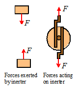 The ‘Inerter’ is a device that exerts forces
proportional to the relative acceleration
of its two ends. It was invented in
1997 and used in secret by the McLaren Formula 1 racing team to improve the
performance of their cars, but in 2008 was made broadly available (http://www.admin.cam.ac.uk/news/dp/2008081906)
The ‘Inerter’ is a device that exerts forces
proportional to the relative acceleration
of its two ends. It was invented in
1997 and used in secret by the McLaren Formula 1 racing team to improve the
performance of their cars, but in 2008 was made broadly available (http://www.admin.cam.ac.uk/news/dp/2008081906)
The device is so simple
that it is difficult to believe that it has taken over 100 years of vehicle
design to think of it but the secret is really in how to use the
device to design suspensions than in the device itself. The device works by spinning a flywheel
between two moving rods, as sketched in the figure.
The forces exerted by the
ends of the inerter always act along the line of the inerter. The magnitude of the force exerted by an
inerter is given by the formula
where
L is the length, and is the inertia constant of the dashpot.
In the SI system, has units of Ns2/m.
Electrostatic forces
As
an engineer, you will need to be able to design structures and machines that
manage forces. Controlling gravity is,
alas, beyond the capabilities of today’s engineers. It’s also difficult (but
not impossible) to design a spring with a variable stiffness or unstretched
length. But there are forces that you can easily control. Electrostatic and electromagnetic forces are
among the most important ones.
Electrostatic forces are exerted on, and by, charged objects. The concepts of electrical potential, current
and charge are based on experiments. A
detailed discussion of these topics is beyond the scope of this course (it will
be covered in detail in EN51), but electromagnetic and electrostatic forces are
so important in the design of engines and machines that the main rules
governing forces in these systems will be summarized here.
Electrostatic forces acting on two small charged
objects that are a large distance apart
 Coulomb’s Law states that if like charges and are induced on two particles that are a
distance d apart, then particle 1
will experience a force
Coulomb’s Law states that if like charges and are induced on two particles that are a
distance d apart, then particle 1
will experience a force
(acting
away from particle 2), where is a fundamental physical constant known as
the Permittivity of the medium
surrounding the particles (like the Gravitational constant, its value must be
determined by experiment).
In
SI units, are specified in Coulombs, d is in meters, and is the permittivity of free space, with fundamental
units . Permittivity is more usually specified using
derived units, in Farads per meter. The Farad is the unit of capacitance.
The
value of for air is very close to that of a
vacuum. The permittivity of a vacuum is
denoted by .
In SI units its value is approximately
Like gravitational forces,
the electrostatic forces acting on 3D objects with a general distribution of
charge must be determined using complicated calculations. It’s worth giving results for two cases that
arise frequently in engineering designs:
Forces acting between charged flat parallel plates
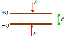
Two parallel plates, which
have equal and opposite charges and are separated by a distance ,
experience an attractive force with magnitude
The force can be thought of
as acting at the center of gravity of the plates.
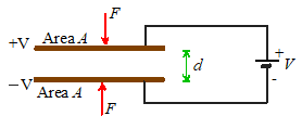 Two parallel plates, which have area A, are separated by a distance d,
and are connected to a power-supply that imposes an electrical potential
difference V across the plates,
experience an attractive force with magnitude
Two parallel plates, which have area A, are separated by a distance d,
and are connected to a power-supply that imposes an electrical potential
difference V across the plates,
experience an attractive force with magnitude
The force can be thought of
as acting at the center of gravity of the plates.
Applications of electrostatic forces:
Electrostatic
forces are small, and don’t have many applications in conventional mechanical
systems. However, they are often used to
construct tiny motors for micro-electro-mechanical
systems (MEMS). The basic idea is to
construct a parallel-plate capacitor, and then to apply force to the machine by
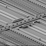
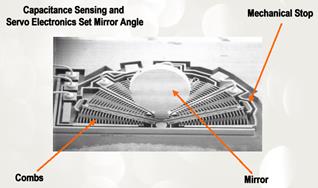
connecting the plates to a power-supply. The pictures below show examples of comb drive motors.
|
|
|
|
An experimental comb drive MEMS actuator developed
at Sandia National Labs, http://mems.sandia.gov/scripts/index.asp
|
A rotary comb drive actuator developed at iolon inc.
Its purpose is to rotate the mirror at the center, which acts as an
optical switch.
|
The
configurations used in practice are basically large numbers of parallel plate
capacitors. A detailed discussion of forces in these systems will be deferred
to future courses.
Electrostatic
forces are also exploited in the design of oscilloscopes, television monitors,
and electron microscopes. These systems
generate charged particles (electrons), for example by heating a tungsten
wire. The electrons are emitted into a
strong electrostatic field, and so are subjected to a large force. The force then causes the particles to
accelerate but we can’t talk about accelerations in this
course so you’ll have to take EN4 to find out what happens next…
Electromagnetic forces
 Electromagnetic forces are exploited more widely than
electrostatic forces, in the design of electric motors, generators, and
electromagnets.
Electromagnetic forces are exploited more widely than
electrostatic forces, in the design of electric motors, generators, and
electromagnets.
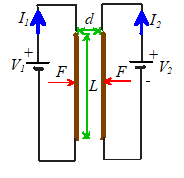
Ampere’s Law
states that two long parallel wires which have length L, carry electric currents and ,
and are a small distance d apart,
will experience an attractive force with magnitude
where is a constant known as the permeability of free space.
In
SI units, has fundamental units of ,
but is usually specified in derived units of Henry per meter. The Henry is the unit of inductance.
The value of is exactly
H/m
Electromagnetic forces
between more generally shaped current carrying wires and magnets are governed
by a complex set of equations. A full
discussion of these physical laws is beyond the scope of this course, and will
be covered in EN51.
Applications of electromagnetic forces
Electromagnetic forces are
widely exploited in the design of electric motors; force actuators; solenoids;
and electromagnets. All these
applications are based upon the principle that a current-carrying wire in a
magnetic field is subject to a force.
The magnetic field can either be induced by a permanent magnet (as in a
DC motor); or can be induced by passing a current through a second wire (used
in some DC motors, and all AC motors).
The general trends of forces in electric motors follow Ampere’s law: the
force exerted by the motor increases linearly with electric current in the
armature; increases roughly in proportion to the length of wire used to wind
the armature, and depends on the geometry of the motor.

Two examples of DC motors the picture on the right is cut open to show
the windings. You can find more
information on motors at http://my.execpc.com/~rhoadley/magmotor.htm
Hydrostatic and buoyancy forces
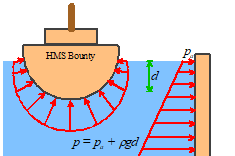 When an object is immersed in a stationary fluid, its
surface is subjected to a pressure. The pressure is actually induced in the fluid
by gravity: the pressure at any depth is effectively supporting the weight of
fluid above that depth.
When an object is immersed in a stationary fluid, its
surface is subjected to a pressure. The pressure is actually induced in the fluid
by gravity: the pressure at any depth is effectively supporting the weight of
fluid above that depth.
A pressure is a distributed force. If a pressure p acts on a surface, a small piece of the surface with area is subjected to a force
where
n is a unit vector perpendicular to
the surface. The total force on a surface must be calculated by
integration. We will show how this is
done shortly.
The pressure in a
stationary fluid varies linearly with depth below the fluid surface
where
is atmospheric pressure (often neglected as
it’s generally small compared with the second term); is the fluid density; g is the acceleration due to gravity; and d is depth below the fluid surface.
Archimedes’ principle gives
a simple way to calculate the resultant force exerted by fluid pressure on an
immersed object.
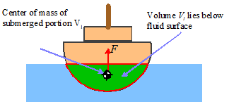
The
magnitude of the resultant force is equal to the weight of water displaced by
the object. The direction is
perpendicular to the fluid surface.
Thus, if the fluid has mass density ,
and a volume of the object lies below the surface of the
fluid, the resultant force due to fluid pressure is
The
force acts at the center of buoyancy
of the immersed object. The center of
buoyancy can be calculated by finding the center of mass of the displaced fluid
(i.e. the center of mass of the portion of the immersed object that lies below
the fluid surface).
The
buoyancy force acts in addition to gravity loading. If the object floats, the gravitational force
is equal and opposite to the buoyancy force.
The force of gravity acts (as usual) at the center of mass of the entire object.
Aerodynamic lift and drag forces
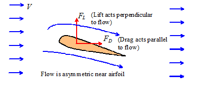 Engineers who design large bridges, buildings, or
fast-moving terrestrial vehicles, spend much time and effort in managing aero-
or hydro-dynamic forces. Hydrodynamic
forces are also of great interest to engineers who design bearings and car
tires, since hydrodynamic forces can cause one surface to float above another,
so reducing friction to very low levels.
Engineers who design large bridges, buildings, or
fast-moving terrestrial vehicles, spend much time and effort in managing aero-
or hydro-dynamic forces. Hydrodynamic
forces are also of great interest to engineers who design bearings and car
tires, since hydrodynamic forces can cause one surface to float above another,
so reducing friction to very low levels.
In general, when air or
fluid flow past an object (or equivalently, if the object moves through
stationary fluid or gas), the object is subjected to two forces:
1.
A Drag force, which acts parallel to the
direction of air or fluid flow
2.
A Lift force, which acts perpendicular to
the direction of air or fluid flow.
The forces act at a point
known as the center of lift of the object but there’s no simple way to predict where
this point is.
The lift force is present
only if airflow past the object is unsymmetrical (i.e. faster above or below
the object). This asymmetry can result
from the shape of the object itself (this effect is exploited in the design of
airplane wings); or because the object is spinning (this effect is exploited by
people who throw, kick, or hit balls for a living).
Two effects contribute to
drag:
(1) Friction between the object’s surface and the fluid or
air. The friction force depends on the
object’s shape and size; on the speed of the flow; and on the viscosity of the fluid, which is a measure
of the shear resistance of the fluid.
Air has a low viscosity; ketchup has a high viscosity. Viscosity is often given the symbol ,
and has the rather strange units in the SI system of .
In `American’ units viscosity has units
of `Poise’ (or sometimes centipoises that’s Poise).
The conversion factor is . (Just
to be confusing, there’s another measure of viscosity, called kinematic viscosity, or specific viscosity, which is ,
where is the mass density of the material. In this course we’ll avoid using kinematic
viscosity, but you should be aware that it exists!) Typical numbers are: Air: for a standard atmosphere (see http://users.wpi.edu/~ierardi/PDF/air_nu_plot.PDF
for a more accurate number) ; Water, ;
SAE40 motor oil ,
ketchup (It’s hard to give a value for the viscosity
of ketchup, because it’s thixotropic.
See if you can find out what this cool word means it’s a handy thing to bring up if you work in
a fast food restaurant.)
(2) Pressure acting on the objects surface. The pressure arises because the air
accelerates as it flows around the object.
The pressure acting on the front of the object is usually bigger than
the pressure behind it, so there’s a resultant drag force. The pressure drag force depends on the
objects shape and size, the speed of the flow, and the fluid’s mass density .
Lift
forces defy a simple explanation, despite the efforts of various authors to
provide one. If you want to watch a
fight, ask two airplane pilots to discuss the origin of lift in your presence. (Of
course, you may not actually know two airplane pilots. If this is the case, and you still want to
watch a fight, you could try http://www.wwe.com/,
or go to a British soccer match). Lift
is caused by a difference in pressure acting at the top and bottom of the object,
but there’s no simple way to explain the origin of this pressure difference. A correct explanation of the origin of lift
forces can be found at http://www.grc.nasa.gov/WWW/K-12/airplane/right2.html
(this site has some neat Java applets that calculate pressure and flow past
airfoils). Unfortunately there are
thousands more books and websites with incorrect explanations of lift, but you
can find those for yourself (check out the explanation from the FAA!)
Lift
and drag forces are usually quantified by defining a coefficient of lift and a coefficient
of drag for the object, and then using the formulas
Here,
is the air or fluid density, V
is the speed of the fluid, and and are measures of the area of the object. Various measures of area are used in practice
when you look up values for drag coefficients
you have to check what’s been used. The object’s
total surface area could be used. Vehicle manufacturers usually use the projected frontal area (equal to car height
x car width for practical purposes) when reporting drag coefficient. and are dimensionless, so they have no units.
The drag and lift
coefficients are not constant, but depend on a number of factors, including:
1. The shape of the object
2. The object’s orientation relative to the flow
(aerodynamicists refer to this as the `angle of attack’)
3. The fluid’s viscosity ,
mass density ,
flow speed V and the object’s size.
Size can be quantified by or ;
other numbers are often used too. For
example, to quantify the drag force acting on a sphere we use its diameter D.
Dimensional analysis shows that and can only depend on these factors through a
dimensionless constant known as `Reynold’s number’, defined as
|
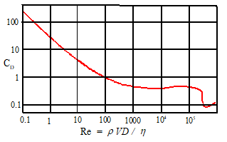
|
|
The
variation of drag coefficient with Reynolds number Re for a smooth sphere.
|
For example, the graph on the right shows the variation
of drag coefficient with Reynolds number for a smooth sphere, with diameter D.
The projected area was used to define the drag coefficient
Many
engineering structures and vehicles operate with Reynolds numbers in the range ,
where drag coefficients are fairly constant (of order 0.01 - 0.5 or so). Lift coefficients for most airfoils are of
order 1 or 2, but can be raised as high as 10 by special techniques such as
blowing air over the wing)
Lift
and drag coefficients can be calculated approximately (you can buy software to
do this for you, e.g. at http://www.hanleyinnovations.com/walite.html
. Another useful resource is www.desktopaero.com/appliedaero ). They usually have to be measured to get really
accurate numbers.
Tables of approximate
values for lift and drag coefficients can be found at http://aerodyn.org/Resources/database.html
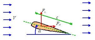
Lift and drag forces are of
great interest to aircraft designers.
Lift and drag forces on an airfoil are computed using the usual formula
The
wing area where c
is the chord of the wing (see the picture) and L is its length, is used in defining both the lift and drag
coefficient.
The
variation of and with angle
of attack are crucial in the design of aircraft. For reasonable values of (below stall - say less than 10 degrees) the
behavior can be approximated by
where
,
and are more or less constant for any given
airfoil shape, for practical ranges of Reynolds number. The first term in the drag coefficient, ,
represents parasite drag due to viscous drag and some pressure
drag. The second term is called induced
drag, and is an undesirable by-product of lift.
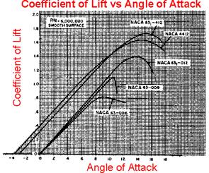
The
graphs on the right, (taken from `Aerodynamics for Naval Aviators, H.H. Hurt,
U.S. Naval Air Systems Command reprint’) shows some experimental data for lift
coefficient as a function of AOA (that’s angle of attack,
but you’re engineers now so you have to talk in code to maximize your nerd
factor. That’s NF). The data suggest that ,
and in fact a simple model known as `thin airfoil theory’ predicts that lift
coefficient should vary by per radian (that works out as 0.1096/degree)
The induced drag
coefficient can be estimated from the formula
where
, L is the length of the wing and c is its width; while e is a constant known as the `Oswald efficiency
factor.’ The constant e is always less than 1 and is of order
0.9 for a high performance wing (eg a jet aircraft or glider) and of order 0.7
for el cheapo wings.
The parasite drag
coefficient is of order 0.05 for the wing of a small
general aviation aircraft, and of order 0.005 or lower for a commercial
airliner.
Interatomic forces
Engineers
working in the fields of nanotechnology, materials design, and bio/chemical
engineering are often interested in calculating the motion of molecules or
atoms in a system.
They
do this using `Molecular Dynamics,’ which is a computer method for integrating
the equations of motion for every atom in the solid. The equations of motion are just Newton’s law F=ma for each atom but for the method to work, it is necessary to
calculate the forces acting on the atoms.
Specifying these forces is usually the most difficult part of the
calculation.
The forces are computed
using empirical force laws, which are either determined experimentally, or
(more often) by means of quantum-mechanical calculations. In the simplest models, the atoms are assumed
to interact through pair forces. In this
case
·
The forces
exerted by two interacting atoms depends only on their relative positions, and
is independent on the position of other atoms in the solid
·
The forces act
along the line connecting the atoms.
·
The magnitude of
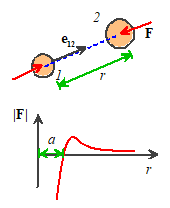
the force is a function of the distance between them. The function is chosen so that (i) the force
is repulsive when the atoms are close together; (ii) the force is zero at the
equilibrium interatomic spacing; (iii) there is some critical distance where
the attractive force has its maximum value (see the figure) and (iv) the force
drops to zero when the atoms are far apart.
Various
functions are used to specify the detailed shape of the force-separation
law. A common one is the so-called
‘Lennard Jones’ function, which gives the force acting on atom (1) as
Here a is the equilibrium separation between the atoms, and E is the total bond energy the amount of work required to separate the
bond by stretching it from initial length a
to infinity.
This
function was originally intended to model the atoms in a Noble gas like He or Ar, etc. It is sometimes used in simple models of
liquids and glasses. It would not be a
good model of a metal, or covalently bonded solids. In fact, for these materials pair potentials
don’t work well, because the force exerted between two atoms depends not just
on the relative positions of the two atoms themselves, but also on the
positions of other nearby atoms. More
complicated functions exist that can account for this kind of behavior, but
there is still a great deal of uncertainty in the choice of function for a particular
material.
2.2 Moments
The
moment of a force is a measure of its tendency to rotate an object about
some point. The physical significance of
a moment will be discussed later. We
begin by stating the mathematical definition of the moment of a force about a
point.
2.2.1
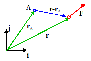
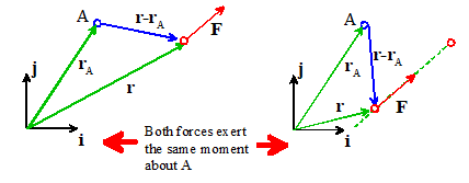
Definition of the moment of a force.
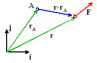 To calculate the moment of a force about some point,
we need to know three things:
To calculate the moment of a force about some point,
we need to know three things:
1. The force vector, expressed as components in a basis ,
or better as
2. The position vector (relative to some convenient
origin) of the point where the force is acting or better
3. The position vector of the point (say point A)
we wish to take moments about (you must use the same origin as for 2) or
The moment of F
about point A is then defined as
We
can write out the formula for the components of in longhand by using the definition of a cross
product
The moment of F about
the origin is a bit simpler
or, in terms of components
2.2.2 Resultant moment exerted by a force system.
Suppose
that N forces act at positions . The resultant
moment of the force system is simply
the sum of the moments exerted by the forces.
You can calculate the resultant moment by first calculating the moment
of each force, and then adding all the moments together (using vector sums).
Just one word of caution is
in order here when you
compute the resultant moment, you must take moments about the same point for
every force.
Taking moments about a
different point for each force and adding the result is meaningless!
2.2.3
Examples of moment calculations using the vector formulas
We work through a few
examples of moment calculations
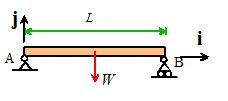
Example 1: The beam shown
below is uniform and has weight W.
Calculate the moment exerted by the gravitational force about points A and B.
We
know (from the table provided earlier) that the center of gravity is half-way
along the beam.
The force (as a vector) is
To
calculate the moment about A, we take the origin at A. The position vector of
the force relative to A is
The moment about A
therefore
To calculate the moment
about B, we take B as the origin. The
position vector of the force relative to B is
Therefore
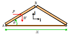 Example 2. Member
AB of a roof-truss is subjected
to a vertical gravitational force W
and a horizontal wind load P. Calculate the moment of the resultant force
about B.
Example 2. Member
AB of a roof-truss is subjected
to a vertical gravitational force W
and a horizontal wind load P. Calculate the moment of the resultant force
about B.
Both the wind load and
weight act at the center of gravity.
Geometry shows that the position vector of the CG with respect to B is
The resultant force is
Therefore the moment about
B is
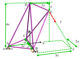 Example 3. The structure
shown is subjected to a force T
acting at E along the line EF.
Calculate the moment of T
about points A and D.
Example 3. The structure
shown is subjected to a force T
acting at E along the line EF.
Calculate the moment of T
about points A and D.
This example requires a lot more work. First we need to write down the force as a
vector. We know the magnitude of the
force is T, so we only need to work
out its direction. Since the force acts
along EF, the direction must be a unit vector pointing along EF.
It’s not hard to see that the vector EF
is
We can divide by the length
of EF ( ) to find a unit vector pointing in the
correct direction
The force vector is
Next, we need to write down
the necessary position vectors
Force:
Point
A:
Point
D:
Finally, we can work
through the necessary cross products
Clearly,
vector notation is very helpful when solving 3D problems!
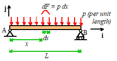 Example 4. Finally, we work through a
simple problem involving distributed
loading. Calculate expressions for the
moments exerted by the pressure acting on the beam about points A and B.
Example 4. Finally, we work through a
simple problem involving distributed
loading. Calculate expressions for the
moments exerted by the pressure acting on the beam about points A and B.
An
arbitrary strip of the beam with length dx
is subjected to a force
The
position vector of the strip relative to A is
The
force acting on the strip therefore exerts a moment
The
total moment follows by summing (integrating) the forces over the entire length
of the beam
The
position vector of the strip relative to B is
The
force acting on the strip exerts a moment
The
total moment follows by summing (integrating) the forces over the entire length
of the beam
2.2.4
The Physical Significance of a Moment
A force acting on a solid
object has two effects: (i) it tends to accelerate the object (making the
object’s center of mass move); and (ii) it tends to cause the object to rotate.
1.
The moment of
a force about some point quantifies its tendency to rotate an object about that
point.
2.
The
magnitude of the moment specifies the magnitude of the rotational force.
3.
The direction
of a moment specifies the axis of rotation associated with the rotational
force, following the right hand screw convention.
Let’s explore these
statements in more detail.
The
best way to understand the physical significance of a moment is to think about
the simple experiments you did with levers & weights back in
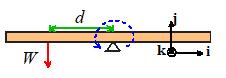
kindergarten. Consider a beam that’s
pivoted about some point (e.g. a see-saw).
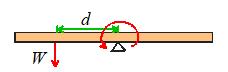
Hang a weight W at
some distance d to the left of the pivot, and the beam will rotate
(counter-clockwise)
To stop the beam rotating,
we need to hang a weight on the right side of the pivot. We could
(a)
Hang a weight W
a distance d to the right of the pivot
(b)
Hang a weight 2W
a distance d/2 to the right of the pivot
(c)
Hang a weight W/2
a distance 2d to the right of the pivot
(d)
Hang a weight a distance to the right of the pivot.
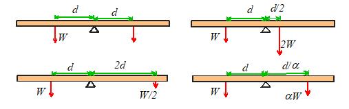
Four ways to balance the beam
These
simple experiments suggest that the turning tendency of a force about some
point is equal to the distance from the point multiplied by the force. This is certainly consistent with
 To see where the cross product in the definition comes
from, we need to do a rather more sophisticated experiment. Let’s now apply a force F at a
distance d from the pivot, but now instead of making the force act
perpendicular to the pivot, let’s make it act at some angle. Does this have a
turning tendency Fd?
To see where the cross product in the definition comes
from, we need to do a rather more sophisticated experiment. Let’s now apply a force F at a
distance d from the pivot, but now instead of making the force act
perpendicular to the pivot, let’s make it act at some angle. Does this have a
turning tendency Fd?
A
little reflection shows that this cannot be the case. The force F can be split into two
components perpendicular to the beam, and parallel to it. But the component parallel to the beam will
not tend to turn the beam. The turning
tendency is only .
Let’s compare this with . Take the origin at the pivot, then
so the magnitude of the
moment correctly gives the magnitude of the turning tendency of the force. That’s why the definition of a moment needs a
cross product.
Finally we need to think
about the significance of the direction of the moment. We can get some insight by calculating for forces acting on our beam to the right and
left of the pivot
For the
force acting on the left of the pivot, we just found
For the force acting on the
right of the pivot
Thus, the force on the left
exerts a moment along the +k direction, while the force on the right
exerts a moment in the k
direction.
Notice
also that the force on the left causes counterclockwise rotation; the force on
the right causes clockwise rotation.
Clearly, the direction of the moment has something to do with the
direction of the turning tendency.
Specifically,
the direction of a moment specifies the axis associated with the rotational
force, following the right hand screw convention.
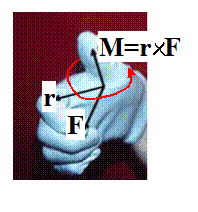
It’s
best to use the screw rule to visualize the effect of a moment hold your right hand as shown, with the thumb
pointing along the direction of the moment.
Your curling fingers (moving from your palm to the finger tips) then
indicate the rotational tendency associated with the moment. Try this for the beam problem. With your thumb pointing along +k (out
of the picture), your fingers curl counterclockwise. With your thumb pointing along k, your
fingers curl clockwise.
2.2.5 A few tips on
calculating moments
 The safest way to calculate the moment of a force is
to slog through the formula, as described at the start of this
section. As long as you can write down
position vectors and force vectors correctly, and can do a cross product, it is
totally fool-proof.
The safest way to calculate the moment of a force is
to slog through the formula, as described at the start of this
section. As long as you can write down
position vectors and force vectors correctly, and can do a cross product, it is
totally fool-proof.
But if you have a good
physical feel for forces and their effects you might like to make use of the
following short cuts.
1. The direction of a
moment is always perpendicular to both and F. For 2D problems, and F lie in the same plane,
so the direction of the moment must be perpendicular to this plane.
Thus, a set of 2D forces in
the {i,j} plane can only exert moments in the direction this makes calculating moments in 2D problems
rather simple; we just have to figure out whether the sign of a moment is
positive or negative.
You can do a quick
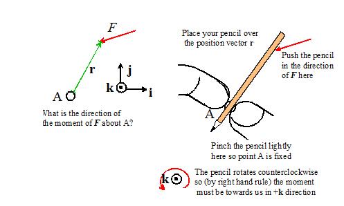
experiment to see whether the direction is +k or k. Suppose you want to find the direction of
the moment caused by F in the picture above about the point A. To do so,
(i)
Place your pencil
on the page so that it lies on the line connecting A to the force.
(ii)
Pinch the pencil
lightly at A so it can rotate about A, but A remains fixed.
(iii)
Push on the
pencil in the direction of the force at B.
If the pencil rotates counterclockwise, the direction of the moment of F
about A is out of the picture (usually +k). If it rotates clockwise, the direction of the
moment is into the picture (k). If it doesn’t rotate, you’re either
holding the pencil in a death grip at A (then the experiment won’t work) or
else the force must be acting along the pencil
in this case the moment is zero.
In
practice you will soon find that you can very quickly tell the direction of a
moment (in 2D, anyway) just by looking at the picture, but the experiment might
help until you develop this intuition.
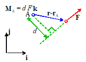
2.
The magnitude of a moment about some point is equal to the perpendicular
distance from that point to the line of action of the force, multiplied by the
magnitude of the force.
Again,
this trick is most helpful in 2D. Its
use is best illustrated by example.
Let’s work through the simple 2D example problems again, but now use the
short-cut.
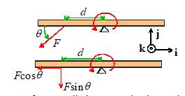
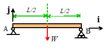 Example 1: The beam shown below is uniform and has
weight W. Calculate the moment exerted
by the gravitational force about points A and B.
Example 1: The beam shown below is uniform and has
weight W. Calculate the moment exerted
by the gravitational force about points A and B.
The perpendicular distance
from a vertical line through the CG to A is L/2. The pencil trick shows that W exerts a clockwise moment about
A. Therefore
Similarly, the perpendicular
distance to B is L/2, and W exerts a counterclockwise moment about
B. Therefore
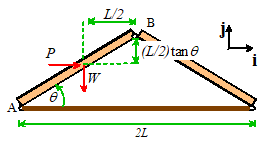 Example 2.
Member AB
of a roof-truss is subjected to a vertical gravitational force W and a horizontal wind load P.
Calculate the moment of the resultant force about B.
Example 2.
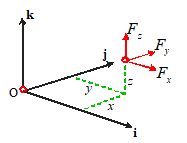
Member AB
of a roof-truss is subjected to a vertical gravitational force W and a horizontal wind load P.
Calculate the moment of the resultant force about B.
The perpendicular distance
from the line of action of W to B is L/2.
W exerts a counterclockwise
moment about B. Therefore W exerts a moment
The perpendicular distance
from the line of action of P to B is . P
also exerts a counterclockwise moment about B.
Therefore
The total moment is
 Example
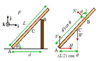
3: It is traditional in
elementary statics courses to solve lots of problems involving ladders (oh boy!
Aren’t you glad you signed up for engineering?) . The picture below shows a ladder of length L
and weight W resting on the top of a frictionless wall. Forces acting on
the ladder are shown as well. Calculate the moments about point A of the
reaction force at B (which acts perpendicular to the ladder) and the weight
force at C (which acts at the center of gravity, half-way up the ladder).
Example
3: It is traditional in
elementary statics courses to solve lots of problems involving ladders (oh boy!
Aren’t you glad you signed up for engineering?) . The picture below shows a ladder of length L
and weight W resting on the top of a frictionless wall. Forces acting on
the ladder are shown as well. Calculate the moments about point A of the
reaction force at B (which acts perpendicular to the ladder) and the weight
force at C (which acts at the center of gravity, half-way up the ladder).
The perpendicular distance
from point A to the line along which N acts is . The pencil experiment (or inspection) shows
that the direction of the moment of N about A is in the +k
direction. Therefore the trick
(perpendicular distance times force) gives
The perpendicular distance
from point A to the line along which W is acting is . The direction of the moment is k. Therefore
Let’s compare these with
the answer we get using . We can take the origin to be at A to make things simple. Then, for the force at B
giving the same answer as
before, but with a whole lot more effort!
Similarly, for the weight
force
3.
The moment exerted by a force is unchanged if the force is moved in a
direction parallel to the direction of the force.
This
is rather obvious in light of trick (2), but it’s worth stating anyway.
4.
The component of moment exerted by a force about an axis through a point can
be calculated by (i) finding the two force components perpendicular to the
axis; then (ii) multiplying each force component by its perpendicular distance
from the axis; and (iii) adding the contributions of each force component
following the right-hand screw convention.
The wording of this one
probably loses you, so let’s start by trying to explain what this means.
First, let’s review what we
mean by the component of a moment about some axis. The formula for the moment of a force about
the origin is
This has three components -
about the i axis, about the j axis, and about the k axis.
The
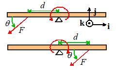
trick gives you a quick way to calculate one of the components. For example, let’s try to find the i
component of the moment about the origin exerted by the force shown in the
picture.
The rule says
(i)
Identify the
force components perpendicular to the i axis that’s and in this case;
(ii)
Multiply each
force component by its perpendicular distance from the axis. Drawing a view down the i axis is
helpful. From the picture, we can see
that is a distance y from the axis, and is a distance z from the axis. The two contributions we need are thus and .
(iii)
 Add the two contributions according to the right hand
screw rule. We know that each force
component exerts a moment - we have to figure out which one is +i and
which is i. We can do the pencil experiment to figure
this out the answer is that exerts a moment along +i, while causes a moment along i. So finally .
Add the two contributions according to the right hand
screw rule. We know that each force
component exerts a moment - we have to figure out which one is +i and
which is i. We can do the pencil experiment to figure
this out the answer is that exerts a moment along +i, while causes a moment along i. So finally .
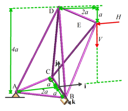
Example: The structure shown is subjected to a vertical force V and horizontal force H acting at E. Calculate the k component of moment exerted about
point A by the resultant force.
Our
trick gives the answer immediately.
First, draw a picture looking down the k axis
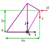
Clearly, the force H
exerts a k component of moment ,
while the force V exerts a k component of moment . The total k component of moment is
This trick clearly can save a great deal of time. But to make use of it, you need excellent 3D
visualization skills.
2.3 Force Couples, Pure Moments, Couples and Torques
We
have seen that a force acting on a rigid body has two effects: (i) it tends to
move the body; and (ii) it tends to rotate the body.
A natural question arises is there a way to rotate a body without moving
it? And is there a kind of force that
causes only rotation without translation?
The answer to both questions
is yes.
2.3.1 Force
couples
 A system of forces that exerts a resultant moment, but
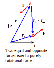
no resultant force, is called a force couple.
A system of forces that exerts a resultant moment, but
no resultant force, is called a force couple.
The
simplest example of a force couple consists of two equal and opposite forces and acting some distance apart. Suppose that the force acts at position while the force acts at position The resultant moment is
Of course, the vector is just the vector from the point where acts to the point where acts.
This gives a quick way to calculate the moment induced by a force
couple:
The
moment induced by two equal and opposite forces is equal to the moment of one
force about the point of action of the other. It doesn’t matter which force
you use to do this calculation.
Note that a force couple
(i)
Has zero
resultant force
(ii)
Exerts the same
resultant moment about all points.
Its effect is to induce
rotation without translation.
The
effect of a force couple can therefore be characterized by a single vector
moment M. The physical
significance of M is equivalent to the physical significance of the
moment of a force about some point. The
direction of M specifies the axis associated with the rotational
force. The magnitude of M
specifies the intensity of the rotational force.
There are many practical examples of force
systems that are best thought of as force-couple systems. They include
- The forces exerted by your hand on a screw-driver
- The forces exerted by the tip of a screw-driver
on the head of a screw
- The forces exerted by one part of a constant
velocity joint on another
- Drag forces acting on a spinning propeller
2.3.2 Pure moments,
couples and torques.- Definition,
Physical Interpretation, and Examples
A pure
moment is a rotational force. Its
effect is to induce rotation, without translation just like a force couple.
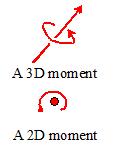
Couples and torques are other
names for a pure moment.
A
pure moment is a vector quantity it has magnitude and direction. The physical significance of the magnitude
and direction of a pure moment are completely equivalent to the moment
associated with a force couple system. The direction of a moment indicates the
axis associated with its rotational force (following the right hand screw
convention); the magnitude represents the intensity of the force. A moment is often denoted by the symbols
shown in the figure.
 The concept of a pure moment takes some getting used
to. Its physical effect can be
visualized by thinking about our beam-balancing problem again.
The concept of a pure moment takes some getting used
to. Its physical effect can be
visualized by thinking about our beam-balancing problem again.
The picture above shows the
un-balanced beam. We saw earlier that we
can balance the beam again by adding a second force, which induces a moment
equal and opposite to that of the force W.
We can also balance the beam
by applying a pure moment to it.
Since the moment of W is ,
a moment applied anywhere on the beam would balance it.
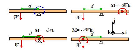
You
could even apply the moment to the left of the beam even right on top of the force W if you
like!
2.3.3 Units and typical
magnitudes of moments
In the SI system, moments
have units of Nm (Newton-meters).
In the US system,
moments have units of ft-lb (foot pounds)
The conversion factor is 1 Nm
= 0.738 ft lb; or 1 ft-lb = 1.356 Nm.
Typical magnitudes are:
- Max torque exerted by a small Lego motor: 0.1 Nm
- Typical torque output of a typical car engine
300-600 Nm
- Breaking torque of a human femur: 140Nm
2.3.4
Measuring Moments

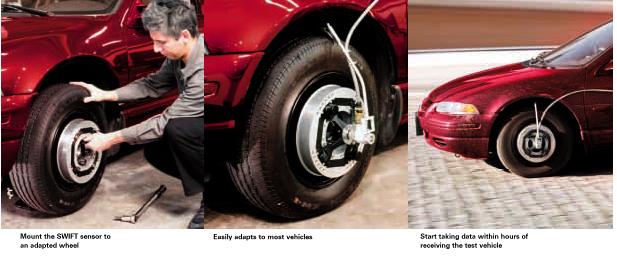
Just as you can buy a force transducer to measure
forces, you can buy a force transducer that measures moments. We showed an example of a force-transducer
attached to the wheel of a car during our earlier discussion of force
transducers.
Another common moment-measuring system is a torque-wrench. (So then is Oprah a talk wench?) When you
tighten the bolts on a precision machine, it’s important to torque them
correctly. If you apply too much torque,
you will strip the thread. If you don’t
apply enough, the bolt will work itself loose during service.
You can buy a tool that measures the moment that you
apply to a bolt while tightening it. The
device may be mechanical, or electronic.
An example (see www.mac.ie/whatwedo/ torquestory.asp ) is shown below.
2.3.5 Engineering systems that exert
torques
There
are many practical examples of moments, or torques, in engineering systems. For
example,
(i)
The driving axle
on your car turns the wheels by exerting a moment on them.
(i)
The drive shaft
of any motor exerts a torque on whatever it’s connected to. In fact, motors are usually rated by their
torque capacity.
(ii)
The purpose of a
gearbox is to amplify or attenuate torque.
You apply a torque to the input shaft, and get a bigger or smaller
torque from the output shaft. To do
this, the input and output shafts have to rotate at different speeds. There are also some clever gearboxes that
allow you to add torques together they are used in split-power variable speed
transmissions, for example.
(iii)
A torque converter serves a similar
purpose to a gearbox. Unlike a gearbox,
however, the input and output shafts don’t rotate at the same speed. The output shaft can be stationary, exerting a
large torque, while the input shaft rotates quickly under a modest torque. It is used as part of an automatic
transmission system in a car.
(iv)
Moments also
appear as reaction forces. For
example, the resistance you feel to turning the steering wheel of your car is
caused by moments acting on the wheels where they touch the ground. The rolling resistance you feel when you ride
your bike over soft ground or grass is also due to a moment acting where the
wheel touches the ground.
(v)
Moments appear as
internal forces in structural members or components. For example, a beam will bend because of an
internal moment whose direction is transverse to the direction of the
beam. A shaft will twist because of an
internal moment whose direction is parallel to the shaft. Just as an internal force causes points in a
solid to move relative to each other, an internal moment causes points to rotate
relative to each other.
2.4 Constraint and reaction forces and moments
Machines
and structures are made up of large numbers of separate components. For example, a building consists of a steel
frame that is responsible for carrying most of the weight of the building and
its contents. The frame is made up of
many separate beams and girders, connected to one another in some way. Similarly, an automobile’s engine and
transmission system contain hundreds of parts, all designed to transmit forces
exerted on the engine’s cylinder heads to the ground.
To
analyze systems like this, we need to know how to think about the forces exerted
by one part of a machine or structure on another.
We
do this by developing a set of rules that specify the forces associated
with various types of joints and connections.
Forces
associated with joints and connections are unlike the forces described in the
preceding section. For all our preceding
examples, (e.g. gravity, lift and drag forces, and so on) we always knew everything
about the forces magnitude, direction, and where the force
acts.
In
contrast, the rules for forces and moments acting at joints and contacts don’t
specify the forces completely. Usually
(but not always), they will specify where the forces act; and they will
specify that the forces and moments can only act along certain directions. The magnitude of the force is always
unknown.
2.4.1 Constraint forces:
overview of general nature of constraint forces
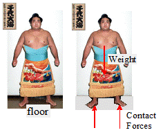 The general nature of a contact force is nicely
illustrated by a familiar example a person, standing on a floor (a Sumo wrestler
was selected as a model, since they are particularly interested in making sure
they remain in contact with a floor!).
You know the floor exerts a force on you (and you must exert an equal
force on the floor). If the floor is
slippery, you know that the force on you acts perpendicular to the floor, but
you can’t make any measurements on the properties of the floor or your feet to
determine what the force will be.
The general nature of a contact force is nicely
illustrated by a familiar example a person, standing on a floor (a Sumo wrestler
was selected as a model, since they are particularly interested in making sure
they remain in contact with a floor!).
You know the floor exerts a force on you (and you must exert an equal
force on the floor). If the floor is
slippery, you know that the force on you acts perpendicular to the floor, but
you can’t make any measurements on the properties of the floor or your feet to
determine what the force will be.
In
fact, the floor will always exert on your feet whatever force is necessary
to stop them sinking through the floor.
(This is generally considered to be a good thing, although there are
occasions when it would be helpful to be able to break this law).
We
can of course deduce the magnitude of the force, by noting that since you don’t
sink through the floor, you are in equilibrium (according to Newton’s definition anyway you may be far from equilibrium
mentally). Let’s say you weight 300lb
(if you don’t, a visit to Dunkin Donuts will help you reach this weight). Since the only forces acting on you are
gravity and the contact force, the resultant of the contact force must be equal
and opposite to the force of gravity to ensure that the forces on you sum to
zero. The magnitude of the total contact force is therefore 300lb. In addition,
the resultant of the contact force must act along a line passing through your
center of gravity, to ensure that the moments on you sum to zero.
From
this specific example, we can draw the following general rules regarding
contact and joint forces
(1) All contacts and joints impose constraints on
the relative motion of the touching or connected components that is to say, they allow only certain types
of relative motion at the joint. (e.g. the floor imposes the constraint that
your feet don’t sink into it)
(2) Equal and opposite forces and moments act on the two
connected or contacting objects. This
means that for all intents and purposes, a
constraint force acts in more than one direction at the same time. This is perhaps the most confusing feature of
constraint forces.
(3) The direction of the forces and moments acting on the
connected objects must be consistent with the allowable relative motion at the
joint (detailed explanation below)
(4) The magnitude of the forces acting at a joint or
contact is always unknown. It can sometimes
be calculated by considering equilibrium (or for dynamic problems, the
motion) of the two contacting parts (detailed explanation later).
Because forces acting at
joints impose constraints on motion, they are often called constraint
forces.
They are also called reaction
forces, because the joints react to impose restrictions on the
relative motion of the two contacting parts.
2.4.2 How to determine
directions of reaction forces and moments at a joint
Let’s
explore the meaning of statement (3) above in more detail, with some specific
examples.
In
our discussion of your interaction with a slippery floor, we stated that the
force exerted on you by the floor had to be perpendicular to the floor. How do we know this?
Because,
according to (3) above, forces at the contact have to be consistent with the
nature of relative motion at the contact or joint. If you stand on a slippery floor, we know
(1) You can slide freely in any direction parallel to the
floor. That means there can’t be a force
acting parallel to the floor.
(2) If someone were to grab hold of your head and try to
spin you around, you’d rotate freely; if someone were to try to tip you over,
you’d topple. Consequently, there can’t be any moment acting on you.
(3) You are prevented from sinking vertically into the
floor. A force must act to prevent this.
(4) You can remove your feet from the floor without any
resistance. Consequently, the floor can
only exert a repulsive force on you, it can’t attract you.
You
can use similar arguments to deduce the forces associated with any kind of
joint. Each time you meet a new kind of
joint, you should ask
(1) Does the connection allow the two connected solids
move relative to each other? If so, what
is the direction of motion? There can be no component of reaction force along
the direction of relative motion.
(2) Does the connection allow the two connected solids
rotate relative to each other? If so,
what is the axis of relative rotation?
There can be no component of reaction moment parallel to the axis of
relative rotation.
(3) For certain types of joint, a more appropriate
question may be ‘Is it really healthy/legal for me to smoke this?’
2.4.3 Drawing free body
diagrams with constraint forces
When
we solve problems with constraints, we are nearly always interested in
analyzing forces in a structure containing many parts, or the motion of a
machine with a number of separate moving components. Solving this kind of problem is not
difficult but it is very complicated because of the
large number of forces involved and the large number of equations that must be
solved to determine them. To avoid
making mistakes, it is critical to use a systematic, and logical, procedure for
drawing free body diagrams and labeling forces.
The
procedure is best illustrated by means of some simple Mickey Mouse
examples. When drawing free body
diagrams yourself, you will find it helpful to consult Section 4.3.4 for the
nature of reaction forces associated with various constraints.
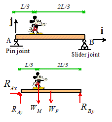
2D Mickey-mouse problem 1. The figure shows Mickey Mouse standing on a beam
supported by a pin joint at one end and a slider joint at the other.
We consider Mickey and the
floor together as the system of interest.
We draw a picture of the system, isolated from its surroundings
(disconnect all the joints, remove contacts, etc). In the picture, all the joints and
connections are replaced by forces, following the rules outlined in the
preceding section.
Notice
how we’ve introduced variables to denote the unknown force components. It is sensible to use a convention that
allows you to quickly identify both the position and direction associated with
each variable. It is a good idea to use
double subscripts the first subscript shows where the
force acts, the second shows its direction.
Forces are always taken to be positive if they act along the
positive x, y and z directions.
We’ve
used the fact that A is a pin joint, and therefore exerts both vertical and
horizontal forces; while B is a roller joint, and exerts only a vertical
force. Note that we always, always draw all admissible forces on the FBD, even
if we suspect that some components may turn out later to be zero. For example, it’s fairly clear that in this example, but it would be incorrect to
leave off this force. This is especially
important in dynamics problems where your intuition regarding forces is very
often incorrect.
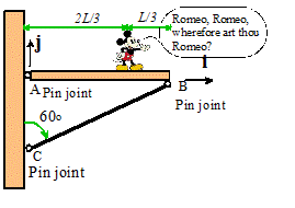 2D Mickey Mouse problem 2 Mickey mouse of weight stands on a balcony of weight as shown.
The weight of strut CB may be neglected.
2D Mickey Mouse problem 2 Mickey mouse of weight stands on a balcony of weight as shown.
The weight of strut CB may be neglected.
This
time we need to deal with a structure that has two parts connected by a joint
(the strut BC is connected to the floor AB through a pin joint). In cases like this you have a choice of (a)
treating the two parts together as a single system; or (b) considering the
strut and floor as two separate systems.
As an exercise, we will draw free body diagrams for both here.
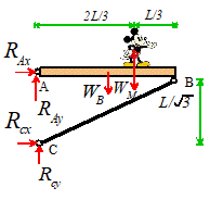
A
free body diagram for the balcony and strut together is shown on the right. Note again the convention used to denote the
reactions: the first label denotes the location of the force, the second
denotes the direction. Both A and C are
pin joints, and therefore exert both horizontal and vertical forces.
The picture shows free body
diagrams for both components. Note the
convention we’ve introduced to deal with the reaction force acting at B it’s important to use a systematic way to deal
with forces exerted by one component in a system on another, or you can get
hopelessly confused. The recommended
procedure is
1. 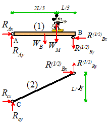 Label the components with numbers here the balcony is (1) and the strut is (2)
2. Denote reaction forces acting between components with
the following convention. In the symbol ,
the superscript (1/2) denotes that the variable signifies the force exerted by
component (1) on component (2) (it’s easy to remember that (1/2) is
1 on 2). The subscript Bx denotes
that the force acts at B, and it acts in the positive x direction.
3.
The forces ,
exerted by component (1) on component (2) are
drawn in the positive x and y directions on the free body diagram
for component (2).
4. The forces exerted by component (2) on component (1)
are equal and opposite to ,
. They are therefore drawn in the negative x
and y directions on the free body diagram for component (1). You need to think of the reaction force
components as acting in two directions at
the same time. This is confusing,
but that’s the way life is.
 2.4.4 Reaction Forces and Moments associated with
various types of joint
2.4.4 Reaction Forces and Moments associated with
various types of joint
Clamped, or welded
joints
No relative motion or
rotation is possible.
Reaction forces: No relative motion is possible in any direction. Three components of reaction force must be
present to prevent motion in all three directions.
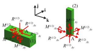 Reaction
moments: No relative rotation is
possible about any axis. Three
components of moment must be present to prevent relative rotation.
Reaction
moments: No relative rotation is
possible about any axis. Three
components of moment must be present to prevent relative rotation.
The figure shows reaction forces acting on the two
connected components. The forces and
moments are labeled according to the conventions described in the preceding
section.
2D versions of the clamped
joint are shown below
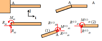
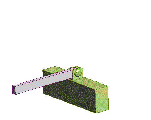 Pinned joint.
A
pinned joint is like a door hinge, or the joint of your elbow. It allows rotation about one axis, but
prevents all other relative motion.
Reaction forces: No relative motion is possible at the joint. There must be 3 components of reaction force
acting to prevent motion.
Reaction moments: Relative rotation is possible about one axis
(perpendicular to the hinge) but is prevented about axes perpendicular to the
hinge. There must be two components of
moment acting at the joint.
2D pinned joints are often
represented as shown in the picture below
Roller and journal
bearings
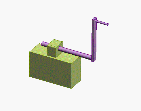 Bearings are used to support rotating shafts. You can buy many different kinds of bearing,
which constrain the shaft in different ways. We’ll look at a couple of different ones.
Bearings are used to support rotating shafts. You can buy many different kinds of bearing,
which constrain the shaft in different ways. We’ll look at a couple of different ones.
Example 1: The bearing shown below is like a pin joint: it
allows rotation about one axis, but prevent rotation about the other two, and
prevents all relative displacement of the shaft.
Reaction forces: No relative motion is possible at this kind of bearing. There must be 3 components of reaction force.
Reaction moments: Relative rotation is allowed about one axis (parallel
to the shaft), but prevented about the other two. There must be two components of reaction
moment.
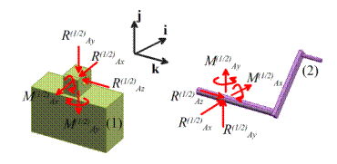
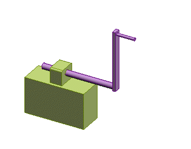 Example2: Some types of
bearing allow the shaft both to rotate, and to slide through the bearing as
shown below
Example2: Some types of
bearing allow the shaft both to rotate, and to slide through the bearing as
shown below
Reaction forces: No relative motion is possible transverse to the
shaft, but the shaft can slide freely through the bearing. There must be 2 components of reaction force.
Reaction moments: Relative rotation is allowed about one axis (parallel
to the shaft), but prevented about the other two. There must be two components of reaction
moment.
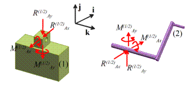
Roller bearings don’t often
appear in 2D problems. When they do,
they look just like a pinned joint.
Swivel joint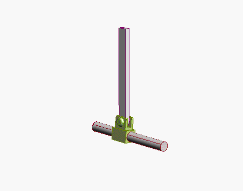 : Like a
pinned joint, but allows rotation about two axes. There must be 3 components of reaction force,
and 1 component of reaction moment.
: Like a
pinned joint, but allows rotation about two axes. There must be 3 components of reaction force,
and 1 component of reaction moment.
Reaction forces: All relative motion is prevented by the joint. There must be three components of reaction
force.
Reaction moments: rotation is permitted about two axes, but prevented about the
third. There must be one component of
reaction force present.
Swivel joints don’t often
appear in 2D problems. When they do,
they look just like a pinned joint.
Ball
and socket joint 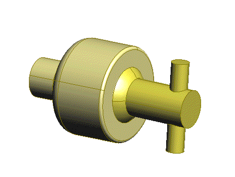 Your hip joint is a good example of a ball and socket
joint. The joint prevents motion, but
allows your thigh to rotate freely relative to the rest of your body.
Your hip joint is a good example of a ball and socket
joint. The joint prevents motion, but
allows your thigh to rotate freely relative to the rest of your body.
Reaction forces: Prevents any relative motion. There must be three components of reaction
force.
Reaction moments. Allows free rotation about all 3 axes. No reaction moments can be present.
Ball joints don’t often
appear in 2D problems. When they do,
they look just like a pinned joint.
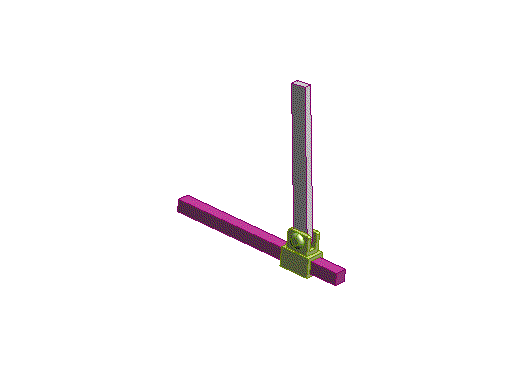 Slider with
pin joint Allows relative motion in
one direction, and allows relative rotation about one axis
Slider with
pin joint Allows relative motion in
one direction, and allows relative rotation about one axis
Reaction forces: Motion is prevented in two directions, but
allowed in the third. There must be two
components of reaction force, acting along directions of constrained motion.
Reaction moments: Relative rotation is prevented about two axes, but allowed about a
third. There must be two components of
reaction moment.
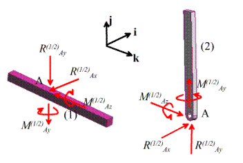
2D slider joints are often
represented as shown in the picture below
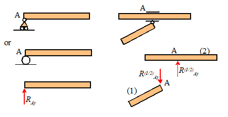
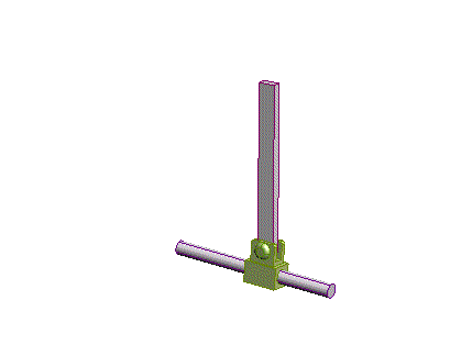
Slider with swivel joint: Similar to a swivel joint, but allows motion in one
direction in addition to rotation about two axes.
Reaction forces: Relative
motion is prevented in two directions, but allowed in the third. There must be two components of reaction
force acting to prevent motion.
Reaction moments: Rotation is permitted around two axes, but prevented around the
third. There must be one component of
reaction moment.
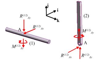
In 2D, a slider with swivel
looks identical to a slider with a pin joint.
2.4.5 Contact Forces
Contacts are actually a bit
more complex than our glib discussion of your interaction with a slippery floor
might suggest.
The nature of the forces
acting at a contact depends on three things:
(1)
Whether the
contact is lubricated, i.e. whether friction acts at the contact
(2)
Whether there is
significant rolling resistance at the contact
(3)
Whether the
contact is conformal, or nonconformal.
A detailed discussion of
friction forces will be left until later.
For now, we will consider only two limiting cases (a) fully lubricated
(frictionless) contacts; and (b) ideally rough (infinite friction) contacts.
Rolling resistance will not
be considered at all in this course.
Forces acting at
frictionless nonconformal contacts
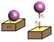
A contact is said to be nonconformal
if the two objects initially touch at a point. The contact between any two convex surfaces
is always non-conformal. Examples
include contact between two balls, a ball and a flat surface, or contact
between two non-parallel cylinders.
The simplest approximation
to the forces acting at a non-conformal lubricated contact states that
(1)
Each solid is
subjected to a force at the contact point;
(2)
The forces
between the two solids are repulsive; this requires and for both examples illustrated in the picture;
(3)
The direction of
the forces are along the line connecting the centers of curvature of the two
contacting surfaces;
(4)
The moments
acting on each solid at the contact point are negligible.
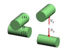
Three rules that help to
establish the direction of frictionless contact forces are:
(1)
When one of the two contacting surfaces is flat, the force must act
perpendicular to the flat surface;
(2)
When two solids contact along sharp edges, the contact force must be
perpendicular to both edges.
(3)
When two curved surfaces contact, the reaction force acts along a line joining
the centers of curvature of the two objects.
Forces acting at rough
(infinite friction) nonconformal
contacts
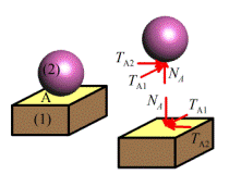
A rough nonconformal
contact behaves somewhat like a pinned joint.
There can be no relative motion of the contacting surfaces, therefore
there must be three components of reaction force acting on both contacting
solids. Unlike a pin joint, however, the
contact can only sustain a repulsive normal force. This means that the
components of force shown in the picture must satisfy . If the normal force is zero (eg when the two
surfaces are about to separate), the tangential forces as well.
The contacting solids can
rotate freely relative to one another.
Therefore there must be no moment acting on the contacting solids at the
point of contact.
Usually the forces acting
at a rough contact are represented by components acting perpendicular and
parallel to the contacting surfaces, as shown in the picture above. If you do this, it’s easy to enforce the constraint.
But if it’s more convenient, you can treat the contact just like a pin
joint, and express the reaction forces in any arbitrary basis, as shown in the
picture below.
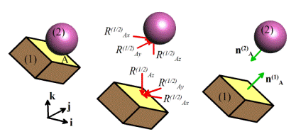
There’s
a minor disadvantage to doing this it’s not easy to check whether the normal
force between the surface is repulsive.
You can do it using vectors for the picture shown the normal force is
repulsive if
Forces acting at
frictionless conformal contacts
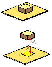 A contact is said to be conformal if two
objects initially contact over a finite area.
Examples include contact between the face of a cube and a flat surface;
contact between the flat end of a cylinder and a flat surface; or a circular
pin inside a matching circular hole.
A contact is said to be conformal if two
objects initially contact over a finite area.
Examples include contact between the face of a cube and a flat surface;
contact between the flat end of a cylinder and a flat surface; or a circular
pin inside a matching circular hole.
Two
conformal solids are actually subjected to a pressure over the area
where they are in contact. It’s really
hard to calculate the pressure distribution (you have to model the deformation
of the two contacting solids), so instead we replace the pressure by a
statically equivalent force.
If the two contacting
surfaces are flat, then
(1)
The reaction
force can be modeled as a single force, with no moment
(2)
The force can act
anywhere within the area of contact (its actual position is determined by force
and moment balance)
(3)
The force must be
perpendicular to the two surfaces
(4)
The force acts to
repel the two solids.
You can of course make
really weird conformal contacts like a jigsaw connection that can completely prevent both relative
translation and rotation of the contacting solids. In this case the contact behaves just like a
clamped joint.
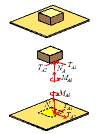 Forces acting at ideally rough (infinite friction)
conformal contacts
Forces acting at ideally rough (infinite friction)
conformal contacts
No
relative motion can occur at the contact.
There must therefore be three components of force acting on each solid.
The
forces can act anywhere within the area of contact (its actual position is determined by force
and moment balance)
The
component of force acting normal to the surface must be repulsive.
No
relative rotation of the two solids can occur. A moment must act about an axis
perpendicular to the contact to prevent relative rotation about this axis.
2.4.6 Some short-cuts for drawing free body diagrams
in systems containing components with negligible mass
The safest procedure in
solving any statics or dynamics problem is to set up and solve equations of
motion for every different part of the structure or machine. There are two particularly common structural
or machine elements that can be treated using short-cuts. These are (i) Two force members in a
structure; and (ii) A freely rotating wheel in a machine.
A Two-force
member is a component or
structural member that
1. 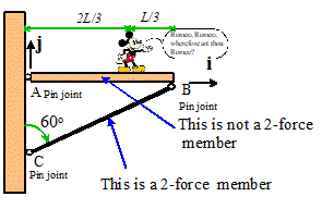 is connected only to two ball-and socket type joints
(in 3D) or pin joints (in 2D).
is connected only to two ball-and socket type joints
(in 3D) or pin joints (in 2D).
2. has negligible weight
We’ve
seen an example already in one of the Mickey Mouse examples it’s shown again in the picture to remind
you. Member BC is
a two-force member, because its weight is negligible, and it has only two pin
joints connecting it to other members. Member AB
is not a two-force member partly because it’s weight is not negligible,
but also because Mickey exerts a force on the member.
The following rules are
very helpful
·
Only one component of reaction force acts at the
joints on a 2-force member
·
The reaction force component acts along a line
connecting the two joints.
It’s trivial to show this if forces act on a body at only two points,
and the body is in static equilibrium, then the forces have to be equal and opposite, and must also act along the same
line, to ensure that both forces and moments are balanced.
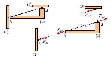
A
generic 2 force member is shown in the figure.
Note that a 2-force member doesn’t have to be straight, though it often
is.
By
convention, a positive reaction force is normally taken to pull at each end of the member, as shown. Equal and opposite reaction forces must act
on whatever is connected to the two force member.
Forces on a freely rotating wheel with
negligible weight: Wheels are so
ubiquitous that it’s worth developing a short-cut to deal with them. The
picture shows a generic 2D wheel, mounted onto an axle with a frictionless bearing.
The contact between wheel and ground is assumed to be ideally rough (infinite
friction).
The following trick is
helpful
For a freely rotating 2D wheel, there is only one
component of reaction force at the contact between the ground and the wheel.
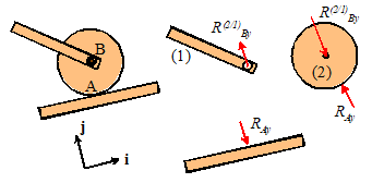 The picture shows a free body diagram for a 2D wheel
mounted on a frictionless bearing.
The picture shows a free body diagram for a 2D wheel
mounted on a frictionless bearing.
Since
only two forces act on the wheel (the force at the axle, and the contact
force), it behaves just like a 2 force member.
The two forces must be equal and opposite, and must act along the same
line. Moreover, the contact force must
satisfy .
For a freely
rotating 3D wheel, there are 2 components of reaction force acting at the
contact between the wheel and ground.
One component acts perpendicular to the ground; the other acts parallel
to the ground and perpendicular to the direction of motion of the wheel (i.e.
parallel to the projection of the wheel’s axle on the ground) .
The picture below shows all
the forces and moments acting on a freely rotating 3D wheel. The reactions that act on the axle are also
shown.
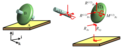
A view from in front of the
wheel shows the directions of the forces and moments more clearly
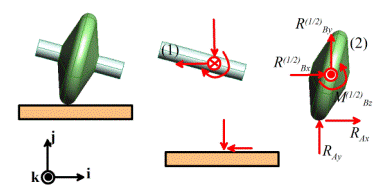
The forces and moments
shown are the only nonzero components of
reaction force.
The
missing force and moment components can be shown to be zero by considering
force and moment balance for the wheel.
The details are left as an exercise.
Finally, a word of caution.
You can
only use these shortcuts if:
1.
The wheel’s weight in negligible;
2.
The wheel rotates freely (no bearing friction, and
nothing driving the wheel);
3.
There is only one contact point on the wheel.
If
any of these conditions are violated you must solve the problem by applying all
the proper reaction forces at contacts and bearings, and drawing a separate
free body diagram for the wheel.
2.5 Friction Forces
Friction
forces act wherever two solids touch. It
is a type of contact force but rather more complicated than the contact
forces we’ve dealt with so far.
It’s
worth reviewing our earlier discussion of contact forces. When we first introduced contact forces, we
said that the nature of the forces acting at a contact depends on three things:
(4)
Whether the
contact is lubricated, i.e. whether friction acts at the contact
(5)
Whether there is
significant rolling resistance at the contact
(6)
Whether the
contact is conformal, or nonconformal.
We
have so far only discussed two types of contact (a) fully lubricated
(frictionless) contacts; and (b) ideally rough (infinite friction) contacts.
Remember
that for a frictionless contact, only one component of force acts on the two
contacting solids, as shown in the picture on the left below. In contrast, for an ideally rough (infinite
friction) contact, three components of force are present as indicated on the
figure on the right.
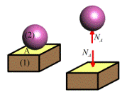
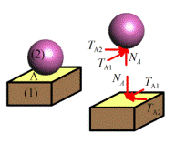
(a)
Reaction forces at a frictionless contact (b) Reaction forces at an ideally
rough contact
All real surfaces lie
somewhere between these two extremes.
The contacting surfaces will experience both a normal and tangential
force. The normal force must be
repulsive, but can have an arbitrary magnitude.
The tangential forces can act in any direction, but their magnitude is
limited. If the tangential forces get
too large, the two contacting surfaces will slip relative to each
other.
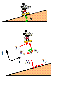
This is why it’s easy to walk up a dry, rough
slope, but very difficult to walk up an icy slope. The picture below helps understand how
friction forces work. The picture shows the big MM walking up a slope with
angle ,
and shows the forces acting on M and the slope.
We can relate the normal and tangential forces acting at the contact to
Mickey’s weight and the angle by doing a force balance
Omitting the tedious details, we find that
Note that a tangential force must act at the contact. If the tangential force gets too large, then
Mickey will start to slip down the slope.
When we do engineering calculations involving
friction forces, we always want to calculate the forces that will cause the two
contacting surfaces to slip. Sometimes
(e.g. when we design moving machinery) we are trying to calculate the forces
that are needed to overcome
friction and keep the parts moving.
Sometimes (e.g. when we design self-locking joints) we need to check
whether the contact can safely support tangential force without sliding.
2.5.1 Experimental measurement of friction forces
To
do both these calculations, we need to know how to determine the critical
tangential forces that cause contacting surfaces to slip. The critical force must be determined
experimentally. Leonardo da Vinci was
apparently the first person to do this his experiments were repeated by Amontons and
Coulomb about 100 years later. We now
refer to the formulas that predict friction forces as Coulomb’s law or
Amonton’s law (you can choose which you prefer!).
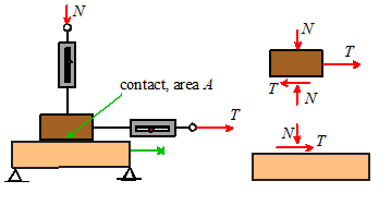 The experiment is conceptually very simple it’s illustrated in the figure.
We put two solids in
contact, and push them together with a normal force N. We then try to slide the two solids relative
to each other by applying a tangential force T. The forces could be measured by force
transducers or spring scales. A simple
equilibrium calculation shows that, as long as the weight of the components can
be neglected, the contacting surfaces must be subject to a normal force N
and a tangential force T.
In an experiment, a normal force would first be
applied to the contact, and then the tangential force would be increased until
the two surfaces start to slip. We could
measure the critical tangential force as a function of N, the area of
contact A, the materials and lubricants involved, the surface finish,
and other variables such as temperature.
You can buy standard
testing equipment for measuring friction forces one configuration is virtually identical to
the simple experiment described above a picture (from http://www.plint-tribology.fsnet.co.uk/cat/at2/leaflet/te75r.htm
) is shown below. This instrument is
used to measure friction between polymeric surfaces.
There are many other techniques for measuring
friction. One common configuration is the `pin on disk’ machine. Two examples
are shown below. The picture on the left
is from www.ist.fhg.de/leistung/gf4/
qualitaet/bildgro4.html , and shows details of the pin and disk. The picture on the right, from www.ulg.ac.be/tribolog/
test.htm shows a pin on disk experiment inside an environmental chamber. In
this test, a pin is pressed with a controlled force onto the surface of a
rotating disk. The force required to
hold the pin stationary is measured.

 Another
test configuration consists of two disks that are pressed into contact and then
rotated with different speeds. The
friction force can be deduced by measuring the torque required to keep the
disks moving. An example (from http://www.ms.ornl.gov/htmlhome/mituc/te53.htm
) is shown below
Another
test configuration consists of two disks that are pressed into contact and then
rotated with different speeds. The
friction force can be deduced by measuring the torque required to keep the
disks moving. An example (from http://www.ms.ornl.gov/htmlhome/mituc/te53.htm
) is shown below
If you want to see a real friction experiment visit
Professor Tullis’ lab
at Brown (you don’t actually have to go there in person; he has a web site
with very detailed descriptions of his lab) he measures friction between rocks, to develop
earthquake prediction models.
A friction experiment must answer two questions:
(i)
What is the critical tangential force that
will cause the surfaces to start to slide? The force required to initiate
sliding is known as the static friction force.
(ii)
If the two surfaces do start to slip, what
tangential force is required to keep
them sliding? The force required to
maintain steady sliding is referred to as the kinetic friction force.
We might guess that the critical force required to
cause sliding could depend on
(i)
The area of contact between the two surfaces
(ii)
The magnitude of the normal force acting at
the contact
(iii)
Surface roughness
(iv)
The nature of the crud on the two surfaces
(v)
What the surfaces are made from
We might also guess that once the surfaces start to
slide, the tangential force needed to maintain sliding will depend on the
sliding velocity, in addition to the variables listed.
In fact, experiments show that
(i) The critical force required to initiate sliding
between surfaces is independent of the area of contact. This is very weird. In fact, when Coulomb first presented this
conclusion to the Academy Francaise, he was thrown out of the room, because the
academy thought that the strength of the contact should increase in proportion
to the contact area. We’ll discuss why
it doesn’t below.
(ii) The critical force required to initiate
sliding between two surfaces is proportional to the normal force. If the normal force is zero, the contact
can’t support any tangential force.
Doubling the normal force will double the critical tangential force that
initiates slip.
(iii) Surface roughness has a very modest effect on
friction. Doubling the surface roughness
might cause only a few percent change in friction force.
(iv) The crud on the two surfaces has a big effect
on friction. Even a little moisture on
the surfaces can reduce friction by 20-30%.
If there’s a thin layer of grease on the surfaces it can cut friction by
a factor of 10. If the crud is removed, friction forces can be huge, and the two
surfaces can seize together completely.
(v) Friction forces depend quite strongly on what
the two surfaces are made from. Some
materials like to bond with each other (metals generally bond well to other
metals, for example) and so have high friction forces. Some materials (e.g. Teflon) don’t bond well
to other materials. In this case
friction forces will be smaller.
(v) If the surfaces start to slide, the tangential
force often (but not always) drops slightly.
Thus, kinetic friction forces are often a little lower than static
friction forces. Otherwise, kinetic
friction forces behave just like static friction they are independent of contact area, are
proportional to the normal force, etc.
(vi) The kinetic friction force usually (but not
always) decreases slightly as the sliding speed increases. Increasing sliding speed by a factor of 10
might drop the friction force by a few percent.
Note that there are some exceptions to these
rules. For example, friction forces
acting on the tip of an atomic force microscope probe will behave completely
differently (but you’ll have to read the scientific literature to find out how
and why!). Also, rubbers don’t behave
like most other materials. Friction
forces between rubber and other materials don’t obey all the rules listed
above.
2.5.2
Definition of friction coefficient: the Coulomb/Amonton friction law
 A
simple mathematical formula known as the Coulomb/Amonton friction law is used
to describe the experimental observations listed in the preceding section.
A
simple mathematical formula known as the Coulomb/Amonton friction law is used
to describe the experimental observations listed in the preceding section.
Friction forces at 2D contacts
Friction forces at a 2D contact are described by
the following laws:
(i) If the two contacting
surfaces do not slide, then
(ii) The two surfaces will start to slip if
(iii) If the two surfaces are sliding, then
The sign in this formula must be selected so that opposes the direction of slip.
In all these formulas, is called the `coefficient of friction’ for the
two contacting materials. For most
engineering contacts, . Actual values are listed below.
Probably we need to
explain statement (iii) in more detail.
Why is there a ? Well, the picture shows the tangential force acting to the right on body (1) and to the
left on body (2). If (1) is stationary
and (2) moves to the right, then this is the correct direction for the force
and we’d use . On the other hand, if (1) were stationary and
(2) moved to the left, then we’d use to make sure that the tangential force acts so
as to oppose sliding.
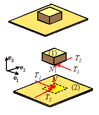
Friction forces at 3D contacts
3D contacts are the same,
but more complicated. The tangential
force can have two components. To
describe this mathematically, we introduce a basis with in the plane of the contact, and normal to the contact. The tangential force exerted by body (1) on body (2) is then
expressed as components in this basis
(i) If the two contacting surfaces do not slide,
then
(ii) The two surfaces will start to slip if
(iii) If the two surfaces are sliding, then
where denotes the tangential force exerted by body
(1) on body (2), and is the relative velocity of body (1) with
respect to body (2) at the point of contact.
The relative velocity can be computed from the velocities and of the two contacting solids, using the
equation .
2.5.3
Experimental values for friction coefficient
The table below (taken from `Engineering Materials’
by Ashby and Jones, Pergammon, 1980) lists rough values for friction
coefficients for various material pairs.
|
Material
|
Approx friction
coefficient
|
|
Clean metals in air
|
0.8-2
|
|
Clean metals in wet air
|
0.5-1.5
|
|
Steel on soft metal (lead, bronze, etc)
|
0.1-0.5
|
|
Steel on ceramics (sapphire, diamond, ice)
|
0.1-0.5
|
|
Ceramics on ceramics (eg carbides on carbides)
|
0.05-0.5
|
|
Polymers on polymers
|
0.05-1.0
|
|
Metals and ceramics on polymers (PE, PTFE, PVC)
|
0.04-0.5
|
|
Boundary lubricated metals (thin layer of grease)
|
0.05-0.2
|
|
High temperature lubricants (eg graphite)
|
0.05-0.2
|
|
Hydrodynamically lubricated surfaces (full oil
film)
|
0.0001-0.0005
|
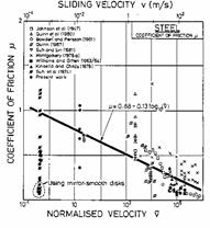 These
are rough guides only friction coefficients for a given material can
by highly variable. For example, Lim and
Ashby (Cambridge University Internal Report CUED/C-mat./TR.123 January 1986)
have catalogued a large number of experimental measurements of friction
coefficient for steel on steel, and present the data graphically as shown
below. You can see that friction
coefficient for steel on steel varies anywhere between 0.0001 to 3.
These
are rough guides only friction coefficients for a given material can
by highly variable. For example, Lim and
Ashby (Cambridge University Internal Report CUED/C-mat./TR.123 January 1986)
have catalogued a large number of experimental measurements of friction
coefficient for steel on steel, and present the data graphically as shown
below. You can see that friction
coefficient for steel on steel varies anywhere between 0.0001 to 3.
Friction coefficient can even vary significantly
during a measurement. For example, the
picture below (from Lim and Ashby, Acta Met 37 3 (1989) p 767) shows the time
variation of friction coefficient during a pin-on-disk experiment.
2.5.4
Static and kinetic friction
Many introductory statics textbooks define two
different friction coefficients. One
value, known as the coefficient of static friction and denoted by ,
is used to model static friction in the equation giving the condition necessary
to initiate slip at a contact
A second value, known as the coefficient of
kinetic friction, and denoted by ,
is used in the equation for the force required to maintain steady sliding
between two surfaces
I don’t like to do this (I’m such a rebel). It is true that for some materials the static
friction force can be a bit higher than the kinetic friction force, but this
behavior is by no means universal, and in any case the difference between and is very small (of the order of 0.05). We’ve already seen that can vary far more than this for a given
material pair, so it doesn’t make much sense to quibble about such a small difference.
The real reason to distinguish between static and
kinetic friction coefficient is to provide a simple explanation for slip-stick
oscillations between two contacting surfaces. Slip-stick oscillations often occur when we
try to do the simple friction experiment shown below.
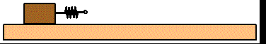
If the end of the spring is moved steadily to the
right, the block sticks for a while until the force in the spring gets large
enough to overcome friction. At this
point, the block jumps to the right and then sticks again, instead of smoothly
following the spring. If were constant, then this behavior would be
impossible. By using ,
we can explain it. But if we’re not
trying to model slip-stick oscillations, it’s much more sensible to work with
just one value of .
In any case, there’s a much better way to model
slip-stick oscillations, by making depend on the velocity of sliding. Most sophisticated models of slip-stick
oscillations (e.g. models of earthquakes at faults) do this.
12.6
The microscopic origin of friction forces
Friction is weird. In particular, we need to explain
(i)
why friction
forces are independent of the contact area
(ii)
why friction
forces are proportional to the normal force.
Coulomb grappled with these
problems and came up with an incorrect explanation. A truly satisfactory explanation for these
observations was only found 20 years or so ago.
To understand friction, we
must take a close look at the nature of surfaces. Coulomb/Amonton friction laws are due to two
properties of surfaces:
(1)
All surfaces are
rough;
(2)
All surfaces are
covered with a thin film of oxide, an adsorbed layer of water, or an organic
film.
 Surface roughness can be controlled to some extent a cast surface is usually very rough; if the
surface is machined the roughness is somewhat less; roughness can be reduced
further by grinding, lapping or polishing the surfaces. But you can’t get rid of it altogether. Many surfaces can be thought of as having a fractal geometry. This means that the
roughness is statistically self-similar with length scale as you zoom in on the surface, it always looks
(statistically) the same (more precisely the surfaces are self-affine. When you zoom
in, it looks like the surface got stretched vertically surfaces are rougher at short wavelengths than
at long ones).
Surface roughness can be controlled to some extent a cast surface is usually very rough; if the
surface is machined the roughness is somewhat less; roughness can be reduced
further by grinding, lapping or polishing the surfaces. But you can’t get rid of it altogether. Many surfaces can be thought of as having a fractal geometry. This means that the
roughness is statistically self-similar with length scale as you zoom in on the surface, it always looks
(statistically) the same (more precisely the surfaces are self-affine. When you zoom
in, it looks like the surface got stretched vertically surfaces are rougher at short wavelengths than
at long ones).
Of course no surface can be
truly fractal: roughness can’t be smaller than the size of an atom and can’t be
larger than the component; but most surfaces look fractal over quite a large
range of lengths. Various statistical
measures are used to quantify surface roughness, but a discussion of these
parameters is beyond the scope of this course.
Now,
visualize what the contact between two rough surfaces looks like. The surfaces will only touch at high spots
(these are known in the trade as `asperities’) on the two surfaces. Experiments suggest that there are huge
numbers of these contacts (nobody has really been able to determine with
certainty how many there actually are).
The asperity tips are squashed flat where they contact, so that there is
a finite total area of contact between the two surfaces. However, the true contact area (at asperity tips) is much smaller than the nominal contact area.
The
true contact area can be estimated by measuring the surface roughness, and then
calculating how the surfaces deform when brought into contact. This is a rather difficult thing to do, but the
best estimates we have today all agree that:
The true area of contact between two rough surfaces is
proportional to the normal force pressing them together.
At present, there is no way
to measure or calculate the contact C
accurately.
This is true for all
materials (except for rubbers, which are so compliant that the true contact
area is close to the nominal contact area), and is just a consequence of the
statistical properties of surface roughness.
The reason that the true contact area increases in proportion to the
load is that as the surfaces are pushed into contact, the number of asperity contacts increases, but the average size of the
contacts remains the same, because of the fractal self-similarity of the two
surfaces.
Finally,
to understand the cause of the Coulomb/Amonton friction law, we need to
visualize what happens when two rough surfaces slide against each other.
Each
asperity tip is covered with a thin layer of oxide, adsorbed water, or
grease. It’s possible to remove this
film in a lab experiment in which case friction behavior changes
dramatically and no longer follows Coulomb/Amonton law but for real engineering surfaces it’s always
present.
The
film usually has a low mechanical strength.
It will start to deform, and so allow the two asperities to slide past
each other, when the tangential force per unit area acting on the film reaches
the shear strength of the film .
The tangential friction
force due to shearing the film on the surface of all the contacting asperities
is therefore
Combining this with the
earlier result for the true contact area gives
Thus,
the friction force is proportional to the normal force. This simple argument also explains why
friction force is independent of contact area; why it is so sensitive to
surface films, and why it can be influenced (albeit only slightly) by surface
roughness.