
Chapter 3
Analyzing motion of systems of particles
In this chapter, we shall discuss
- The concept of a particle
- Position/velocity/acceleration relations for a particle
- How to use
- How to use
- How to solve equations of motion for particles by hand or using a computer.
The focus of this chapter is
on setting up and solving equations of motion we will not discuss in detail the behavior of
the various examples that are solved.
3.1 Equations of motion for a particle
We start with some basic definitions and physical laws.
3.1.1 Definition of a particle
A `Particle’ is a point mass at some position in space. It can move about, but has no characteristic orientation or rotational inertia. It is characterized by its mass.
Examples of applications where you might choose to idealize part of a system as a particle include:
1. Calculating the orbit of a satellite for this application, you don’t need to know
the orientation of the satellite, and you know that the satellite is very small
compared with the dimensions of its orbit.
2. A molecular dynamic simulation, where you wish to calculate the motion of individual atoms in a material. Most of the mass of an atom is usually concentrated in a very small region (the nucleus) in comparison to inter-atomic spacing. It has negligible rotational inertia. This approach is also sometimes used to model entire molecules, but rotational inertia can be important in this case.
Obviously, if you choose to idealize an object as a particle, you will only be able to calculate its position. Its orientation or rotation cannot be computed.
3.1.2 Position, velocity, acceleration relations for a particle (Cartesian coordinates)
 In most practical applications we are interested in
the position or the velocity (or speed) of the particle as a
function of time. But
In most practical applications we are interested in
the position or the velocity (or speed) of the particle as a
function of time. But
Position vector: In most of the problems we solve in this course, we will specify the position of a particle using the Cartesian components of its position vector with respect to a convenient origin. This means
1. We choose three, mutually perpendicular, fixed
directions in space. The three
directions are described by unit vectors
2. We choose a convenient point to use as origin.
3. The position vector (relative to the origin) is then specified by the three distances (x,y,z) shown in the figure.
In dynamics problems, all three components can be functions of time.
Velocity vector: By definition, the velocity is the derivative of the position vector with respect to time (following the usual machinery of calculus)
Velocity is a vector, and can therefore be expressed in terms of its Cartesian components
You can visualize a velocity vector as follows
· The direction of the vector is parallel to the direction of motion
·
The magnitude of the vector is the speed of
the particle (in meters/sec, for example).
When
both position and velocity vectors are expressed in terms Cartesian components,
it is simple to calculate the velocity from the position vector. For this case, the basis vectors are constant
(independent of time) and so
This is really three
equations one for each velocity component, i.e.
Acceleration vector: The acceleration is the derivative of the velocity vector with respect to time; or, equivalently, the second derivative of the position vector with respect to time.
The acceleration is a
vector, with Cartesian representation .
Like
velocity, acceleration has magnitude and direction. Sometimes it may be
possible to visualize an acceleration vector for example, if you know your particle is
moving in a straight line, the acceleration vector must be parallel to the
direction of motion; or if the particle moves around a circle at constant
speed, its acceleration is towards the center of the circle. But sometimes you can’t trust your intuition
regarding the magnitude and direction of acceleration, and it can be best to
simply work through the math.
The relations between Cartesian components of position, velocity and acceleration are
3.1.3 Examples using position-velocity-acceleration relations
It is important for you to be comfortable with calculating velocity and acceleration from the position vector of a particle. You will need to do this in nearly every problem we solve. In this section we provide a few examples. Each example gives a set of formulas that will be useful in practical applications.
Example 1: Constant acceleration along a straight line. There are many examples where an object moves along a straight line, with constant acceleration. Examples include free fall near the surface of a planet (without air resistance), the initial stages of the acceleration of a car, or and aircraft during takeoff roll, or a spacecraft during blastoff.
Suppose that
The particle moves parallel to a unit vector i
The particle has constant acceleration, with magnitude a
At
time the particle has speed
At time the particle has position vector
The position, velocity acceleration vectors are then
Verify for yourself that the position, velocity and acceleration (i) have the correct values at t=0 and (ii) are related by the correct expressions (i.e. differentiate the position and show that you get the correct expression for the velocity, and differentiate the velocity to show that you get the correct expression for the acceleration).
HEALTH WARNING: These results can only
be used if the acceleration is constant.
In many problems acceleration is a function of time, or position in this case these formulas cannot be used.
People who have taken high school physics classes have used these formulas to
solve so many problems that they automatically apply them to everything
this works for high school problems but not always
in real life!
 Example 2: Simple Harmonic Motion: The
vibration of a very simple spring-mass system is an example of simple harmonic motion.
Example 2: Simple Harmonic Motion: The
vibration of a very simple spring-mass system is an example of simple harmonic motion.
In simple harmonic motion (i) the particle moves along a straight line; and (ii) the position, velocity and acceleration are all trigonometric functions of time.
For example, the position vector of the mass might be given by
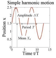
Here
is the average length of the spring,
is the maximum length of the spring, and T is the time for the mass to complete
one complete cycle of oscillation (this is called the `period’ of oscillation).
Harmonic vibrations are also often characterized by the frequency of vibration:
· The frequency in cycles per second (or Hertz) is related to the period by f=1/T
·
The angular frequency is related to the
period by
The motion is plotted in the figure on the right.
The velocity and acceleration can be calculated by differentiating the position, as follows
Note that:
· The velocity and acceleration are also harmonic, and have the same period and frequency as the displacement.
·
If you know the
frequency, and amplitude and of either the displacement, velocity, or
acceleration, you can immediately calculate the amplitudes of the other two. For example, if ,
,
denote the amplitudes of the displacement,
velocity and acceleration, we have that
 Example 3: Motion at constant speed around a circular
path Circular motion is also very common
Example 3: Motion at constant speed around a circular
path Circular motion is also very common examples include any rotating machinery,
vehicles traveling around a circular path, and so on.
The simplest way to make an object move at constant speed along a circular path is to attach it to the end of a shaft (see the figure), and then rotate the shaft at a constant angular rate. Then, notice that
·
The angle increases at constant rate. We can write
,
where
is the (constant)
angular speed of the shaft, in radians/seconds.
·
The speed of the
particle is related to by
. To see this, notice that the circumferential
distance traveled by the particle is
. Therefore,
.
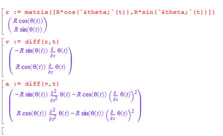
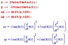
For this example the position vector is
The velocity can be calculated by differentiating the position vector.
Here, we have used the
chain rule of differentiation, and noted that .
The acceleration vector follows as
Note that
(i) The magnitude of the velocity is ,
and its direction is (obviously!) tangent to the path (to see this, visualize
(using trig) the direction of the unit vector
(ii)
The magnitude of the acceleration is and its direction is towards the center of the
circle. To see this, visualize (using trig) the direction of the unit vector
We can write these mathematically as
 Example 4: More general motion around a circular path
We next look at more
general circular motion, where the particle still moves around a circular path,
but does not move at constant speed. The
angle is now a general function of time.
We can write down some useful scalar relations:
·
Angular rate:
·
Angular
acceleration
·
Speed
·
Rate of change of
speed
We can now calculate vector velocities and accelerations
The velocity can be calculated by differentiating the position vector.
The acceleration vector follows as
It is often more convenient
to re-write these in terms of the unit vectors n and t normal and
tangent to the circular path, noting that ,
. Then
These are the famous circular motion formulas that you might have seen in physics class.
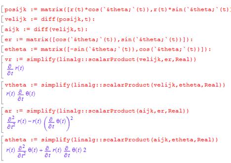
Using MAPLE to differentiate position-velocity-acceleration relations
If
you find that your calculus is a bit rusty you can use MAPLE to do the tedious
work for you. You already know how to
differentiate and integrate in MAPLE the only thing you may not know is how to tell
MAPLE that a variable is a function of time.
Here’s how this works. To
differentiate the vector
you would type
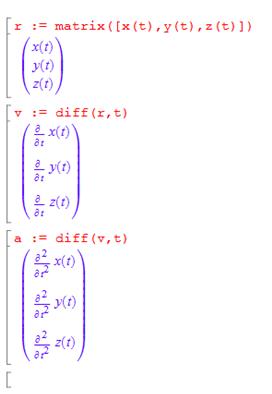
It is essential to type in the (t) after x,y,and z if you don’t do this, Mupad assumes that these
variables are constants, and takes their derivative to be zero. You must enter (t) after _any_ variable that
changes with time.
Here’s
how you would do the circular motion calculation if you only know that the
angle is some arbitrary function of time, but don’t
know what the function is
As
you’ve already seen in EN3, Matlab can make very long and complicated
calculations fairly painless. It is a
godsend to engineers, who generally find that every real-world problem they
need to solve is long and complicated. But
of course it’s important to know what the program is doing so keep taking those math classes…
3.1.4 Velocity and acceleration in normal-tangential and cylindrical polar coordinates.
In
some cases it is helpful to use special basis vectors to write down velocity
and acceleration vectors, instead of a fixed {i,j,k} basis. If you see
that this approach can be used to quickly solve a problem go ahead and use it. If not, just use Cartesian coordinates
this will always work, and with MAPLE is not
very hard. The only benefit of using the
special coordinate systems is to save a couple of lines of rather tedious
trigonometric algebra
which can be extremely helpful when solving an
exam question, but is generally insignificant when solving a real problem.
Normal-tangential coordinates for particles moving along a prescribed planar path
 In some problems, you might know the particle speed,
and the x,y coordinates of the path
(a car traveling along a road is a good example). In this case it is often easiest to use normal-tangential coordinates to
describe forces and motion. For this
purpose we
In some problems, you might know the particle speed,
and the x,y coordinates of the path
(a car traveling along a road is a good example). In this case it is often easiest to use normal-tangential coordinates to
describe forces and motion. For this
purpose we
· Introduce two unit vectors n and t, with t pointing tangent to the path and n pointing normal to the path, towards the center of curvature
· Introduce the radius of curvature of the path R.
If
you happen to know the parametric equation of the path (i.e. the x,y coordinates are known in terms of
some variable ), then
The sign of n should be selected so that
The radius of curvature can be computed from
The radius of curvature is always positive.
The direction of the velocity vector of a particle is tangent to its path. The magnitude of the velocity vector is equal to the speed.
The acceleration vector can be constructed by adding two components:
·
the component of acceleration tangent to the
particle’s path is equal
·
The component of acceleration perpendicular to the path
(towards the center of curvature) is equal to .
Mathematically
 Example: Design speed limit for a curvy road: As
a consulting firm specializing in highway design, we have been asked to develop
a design formula that can be used to calculate the speed limit for cars that
travel along a curvy road.
Example: Design speed limit for a curvy road: As
a consulting firm specializing in highway design, we have been asked to develop
a design formula that can be used to calculate the speed limit for cars that
travel along a curvy road.
The following procedure will be used:
·
The curvy road
will be approximated as a sine wave as shown in the figure
for a given road, engineers will measure
values of A and L that fit the path.
·
Vehicles will be
assumed to travel at constant speed V
around the path your mission is to calculate the value of V
· For safety, the magnitude of the acceleration of the car at any point along the path must be less than 0.2g, where g is the gravitational acceleration. (Again, note that constant speed does not mean constant acceleration, because the car’s direction is changing with time).
Our goal, then, is to calculate a formula for the magnitude of the acceleration in terms of V, A and L. The result can be used to deduce a formula for the speed limit.
Calcluation:
We can solve this problem quickly using normal-tangential coordinates. Since the speed is constant, the acceleration vector is
The
position vector is ,
so we can calculate the radius of curvature from the formula
Note
that x acts as the parameter for this problem, and
,
so
and the acceleration is
We are interested in the magnitude of the acceleration…
We
see from this that the car has the biggest acceleration when .
The maximum acceleration follows as
The
formula for the speed limit is therefore
Now we send in a bill for a big consulting fee…
Polar coordinates for particles moving in a plane
 When solving problems involving central forces (forces
that attract particles towards a fixed point) it is often convenient to
describe motion using polar coordinates.
When solving problems involving central forces (forces
that attract particles towards a fixed point) it is often convenient to
describe motion using polar coordinates.
Polar coordinates are related to x,y coordinates through
Suppose that the position of a particle
is specified by its ‘polar coordinates’ relative to a fixed origin, as shown in the
figure. Let
be a unit vector pointing in the radial
direction, and let
be a unit vector pointing in the tangential
direction, i.e
The velocity and acceleration of the particle can then be expressed as
Deriving
these results takes some tedious algebra, but it’s conceptually simple here’s what we do:
1.
Write down the
position vector in terms of in a fixed (i,j,k) coordinate system
2. Take the time derivatives to find acceleration and velocity in the (i,j,k) coordinate system
3.
Convert the
results to the coordinate system. To do this remember that the component of v parallel to
can be found using a dot product:
. Similarly
Here are the details with Mupad taking care of the tedious algebra.
These are the answers stated.
 Example
The robotic manipulator shown in the figure rotates with constant angular speed
Example
The robotic manipulator shown in the figure rotates with constant angular speed
about the k
axis. Find a formula for the
maximum allowable (constant) rate of extension
if the acceleration of the gripper may not
exceed g.
We
can simply write down the acceleration vector, using polar coordinates. We identify and r=L,
so that
Other examples using polar coordinates can be found in sections below.
3.1.5 Measuring position, velocity and acceleration
If
you are designing a control system, you will need some way to detect the motion of the system you are trying to control. A vast array of different sensors is available
for you to choose from: see for example the list at http://www.sensorland.com/HowPage001.html
. A very short list of common sensors is
given below
the motion of the system you are trying to control. A vast array of different sensors is available
for you to choose from: see for example the list at http://www.sensorland.com/HowPage001.html
. A very short list of common sensors is
given below
1. GPS determines position on the earth’s surface by
measuring the time for electromagnetic waves to travel from satellites in known
positions in space to the sensor. Can
be accurate down to cm distances, but the sensor needs to be left in position
for a long time for this kind of accuracy.
A few m is more common.
2.  Optical or radio frequency position sensing
 measure position by (a) monitoring deflection
of laser beams off a target; or measuring the time for signals to travel from a
set of radio emitters with known positions to the sensor. Precision can vary from cm accuracy down to
light wavelengths.
3. Capacitative displacement sensing determine position by measuring the
capacitance between two parallel plates.
The device needs to be physically connected to the object you are
tracking and a reference point. Can only measure distances of mm or less, but
precision can be down to micron accuracy.
4. Electromagnetic displacement sensing measures position by detecting electromagnetic
fields between conducting coils, or coil/magnet combinations within the
sensor. Needs to be physically connected
to the object you are tracking and a reference point. Measures displacements of order cm down to
microns.
5. Radar velocity sensing measures velocity by detecting the change in
frequency of electromagnetic waves reflected off the traveling object.
6. Inertial accelerometers: measure accelerations by detecting the deflection of a spring acting on a mass.
Accelerometers are also often used to construct an ‘inertial platform,’ which uses gyroscopes to maintain a fixed orientation in space, and has three accelerometers that can detect motion in three mutually perpendicular directions. These accelerations can then be integrated to determine the position. They are used in aircraft, marine applications, and space vehicles where GPS cannot be used.
3.1.6 Newton’s laws of motion for a particle
1. m denote the mass of the particle
2. F denote the resultant force acting on the particle (as a vector)
3. a denote the acceleration of the particle (again, as a vector). Then
Occasionally, we use a particle idealization to model systems which, strictly speaking, are not particles. These are:
1. A large mass, which moves without rotation (e.g. a car moving along a straight line)
2. A single particle which is attached to a rigid frame with negligible mass (e.g. a person on a bicycle)
In these cases it may be necessary to consider the moments acting on the mass (or frame) in order to calculate unknown reaction forces.
1. For a large mass which moves without rotation, the resultant moment of external forces about the center of mass must vanish.
2. For a particle attached to a massless frame, the resultant moment of external forces acting on the frame about the particle must vanish.
It is very important to take moments about the correct point in dynamics problems! Forgetting this is the most common reason to screw up a dynamics problem…
If you need to solve a problem where more than one
particle is attached to a massless frame, you have to draw a separate free body
diagram for each particle, and for the frame.
The particles must obey . The forces acting on the frame must obey
and
,
(because the frame has no mass).
The Newtonian Inertial Frame.
When
we use
For engineering calculations, this usually poses no difficulty. If we are solving problems involving terrestrial motion over short distances compared with the earth’s radius, we simply take a point on the earth’s surface as fixed, and take three directions relative to the earth’s surface to be fixed. If we are solving problems involving motion in space near the earth, or modeling weather, we take the center of the earth as a fixed point, (or for more complex calculations the center of the sun); and choose axes to have a fixed direction relative to nearby stars.
But
in reality, an unambiguous inertial frame does not exist. We can only describe the relative motion of the mass in the universe, not its absolute
motion. The general theory of relativity
addresses this problem and in doing so explains many small but
noticeable discrepancies between the predictions of
It
would be fun to cover the general theory of relativity in this course but regrettably the mathematics needed to
solve any realistic problem is horrendous.
As engineers, we always have to solve realistic problems, and we usually
can’t afford to spend a long time doing complicated calculations, so we use the
simplest theory that will allow us to make the correct design decisions. Newton’s laws are fine for us…
3.2 Calculating forces required to cause prescribed motion of a particle
We use the following general procedure to solve problems like this
(1) Decide how to idealize the system (what are the particles?)
(2) Draw a free body diagram showing the forces acting on each particle
(3) Consider the kinematics
of the problem. The goal is to calculate the acceleration of each particle in
the system you may be able to start by writing down the
position vector and differentiating it, or you may be able to relate the
accelerations of two particles (eg if two particles move together, their
accelerations must be equal).
(4) Write down F=ma for each particle.
(5)
If you are solving a problem involving a massless frames (see, e.g. Example 3,
involving a bicycle with negligible mass) you also need to write down about the particle.
(5) Solve the resulting equations for any unknown components of force or acceleration (this is just like a statics problem, except the right hand side is not zero).
It is best to show how this is done by means of examples.
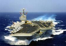 Example 1: Estimate the minimum thrust
that must be produced by the engines of an aircraft in order to take off from
the deck of an aircraft carrier (the figure is from www.lakehurst.navy.mil/NLWeb/media-library.asp)
Example 1: Estimate the minimum thrust
that must be produced by the engines of an aircraft in order to take off from
the deck of an aircraft carrier (the figure is from www.lakehurst.navy.mil/NLWeb/media-library.asp)
We
will estimate the acceleration required to reach takeoff speed, assuming the
aircraft accelerates from zero speed to takeoff speed along the deck of the
carrier, and then use
Data/ Assumptions:
1. The flight deck of a Nimitz class aircraft carrier is about 300m long (http://www.naval-technology.com/projects/nimitz/) but only a fraction of this is used for takeoff (the angled runway is used for landing). We will take the length of the runway to be d=200m
2. We will assume that the acceleration during takeoff roll is constant.
3. We will assume that the aircraft carrier is not moving
(this is wrong actually the aircraft carrier always moves at
high speed during takeoff. We neglect
motion to make the calculation simpler)
4. The FA18 Super Hornet is a typical aircraft used on a
carrier it has max catapult weight of m=15000kg http://www.boeing.com/defense-space/military/fa18ef/docs/EF_overview.pdf
5. The manufacturers are somewhat reticent about
performance specifications for the Hornet but 150 knots (77 m/s) is a reasonable guess for a
minimum controllable airspeed for this aircraft.
Calculations:
1. Idealization: We will idealize the aircraft as a particle. We can do this because the aircraft is not rotating during takeoff.
2.
 FBD: The figure
shows a free body diagram.
FBD: The figure
shows a free body diagram. represents the (unknown) force exerted on the
aircraft due to its engines.
3. Kinematics: We must calculate the acceleration required to reach takeoff speed. We are given (i) the distance to takeoff d, (ii) the takeoff speed and (iii) the aircraft is at rest at the start
of the takeoff roll. We can therefore write down the position vector r and velocity v of the aircraft at takeoff, and use the straight line motion
formulas for r and v to calculate the time t to reach takeoff speed and the
acceleration a. Taking the origin at the initial position of
the aircraft, we have that, at the instant of takeoff
This gives two scalar equations which can be solved for a and t
4. EOM: The vector equation of motion for this problem is
5. Solution: The i component of the equation of motion gives an equation for the unknown force in terms of known quantities
Substituting numbers gives the magnitude of the force as F=222 kN. This is very close, but slightly greater than, the 200kN (44000lb) thrust quoted on the spec sheet for the Hornet. Using a catapult to accelerate the aircraft, speeding up the aircraft carrier, and increasing thrust using an afterburner buys a margin of safety.
 Example 2: Mechanics
of Magic! You have no doubt seen the
simple `tablecloth trick’ in which a tablecloth is whipped out from underneath
a fully set table (if not, you can watch it at http://wm.kusa.gannett.edgestreams.net/news/1132187192333-11-16-05-spangler-2p.wmv)
Example 2: Mechanics
of Magic! You have no doubt seen the
simple `tablecloth trick’ in which a tablecloth is whipped out from underneath
a fully set table (if not, you can watch it at http://wm.kusa.gannett.edgestreams.net/news/1132187192333-11-16-05-spangler-2p.wmv)
In this problem we shall estimate the critical acceleration that must be imposed on the tablecloth to pull it from underneath the objects placed upon it.
We wish to determine conditions for the tablecloth to slip out from under the glass. We can do this by calculating the reaction forces acting between the glass and the tablecloth, and see whether or not slip will occur. It is best to calculate the forces required to make the glass move with the tablecloth (i.e. to prevent slip), and see if these forces are big enough to cause slip.
1. Idealization: We will assume that the glass behaves like a particle (again, we can do this because the glass does not rotate)
2.  FBD. The
figure shows a free body diagram for the glass.
The forces include (i) the weight; and (ii) the normal and tangential
components of reaction at the contact between the tablecloth and the glass. The normal and tangential forces must act
somewhere inside the contact area, but their position is unknown. For a more detailed discussion of contact
forces see Sects 2.4 and 2.5.
FBD. The
figure shows a free body diagram for the glass.
The forces include (i) the weight; and (ii) the normal and tangential
components of reaction at the contact between the tablecloth and the glass. The normal and tangential forces must act
somewhere inside the contact area, but their position is unknown. For a more detailed discussion of contact
forces see Sects 2.4 and 2.5.
3.
Kinematics We are assuming that the glass has the same
acceleration as the tablecloth. The table cloth is moving in the i direction, and has magnitude a. The acceleration vector is therefore .
4.
EOM.
5. Solution: The i and j components of the vector equation must each be satisfied (just as when you solve a statics problem), so that
Finally, we must use the friction law to decide whether or not the tablecloth will slip from under the glass. Recall that, for no slip, the friction force must satisfy
where
is the friction coefficient. Substituting for T and N from (5) shows
that for no slip
To
do the trick, therefore, the acceleration must exceed . For a friction coefficient of order 0.1, this
gives an acceleration of order
. There is a special trick to pulling the
tablecloth with a large acceleration
but that’s a secret.
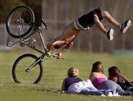 Example 3:
Bicycle Safety. If a bike rider brakes too hard on the front wheel, his
or her bike will tip over (the figure is from http://www.thosefunnypictures.com/picture/7658/bike-flip.html). In this example we investigate the conditions
that will lead the bike to capsize, and identify design variables that can
influence these conditions.
Example 3:
Bicycle Safety. If a bike rider brakes too hard on the front wheel, his
or her bike will tip over (the figure is from http://www.thosefunnypictures.com/picture/7658/bike-flip.html). In this example we investigate the conditions
that will lead the bike to capsize, and identify design variables that can
influence these conditions.
If
the bike tips over, the rear wheel leaves the ground. If this happens, the reaction force acting on
the wheel must be zero so we can detect the point where the bike is
just on the verge of tipping over by calculating the reaction forces, and
finding the conditions where the reaction force on the rear wheel is zero.
1. Idealization:
a. We will idealize the rider as a particle (apologies to
bike racers but that’s how we think of you…). The particle
is located at the center of mass of the rider.
The figure shows the most important design parameters- these are the
height of the rider’s COM, the wheelbase L
and the distance of the COM from the rear wheel.
b. We assume that the bike is a massless frame. The wheels are also assumed to have no
mass. This means that the forces acting
on the wheels must satisfy and
- and can be analyzed using methods of
statics. If you’ve forgotten how to
think about statics of wheels, you should re-read the notes on this topic
in particular, make sure you understand the
nature of the forces acting on a freely rotating wheel (Section 2.4.6 of the
reference notes).
c. We assume that the rider brakes so hard that the front
wheel is prevented from rotating. It
must therefore skid over the ground.
Friction will resist this sliding. We denote the friction coefficient at
the contact point B by .
d. The rear wheel is assumed to rotate freely.
e. We neglect air resistance.
2. FBD. The figure shows a free body diagram for the rider and for the bike together. Note that
a. A normal and tangential force acts at the contact point
on the front wheel (in general, both normal and tangential forces always act at
contact points, unless the contact happens to be frictionless). Because the contact is slipping it is
essential to draw the friction force in the correct direction the force must resist the motion of the bike;
b. Only a normal force acts at the contact point on the rear wheel because it is freely rotating, and behaves like a 2-force member.
3. Kinematics The
bike is moving in the i direction.
As a vector, its acceleration is therefore ,
where a is unknown.
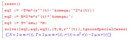
4. EOM: Because
this problem includes a massless frame, we must use two equations of motion ( and
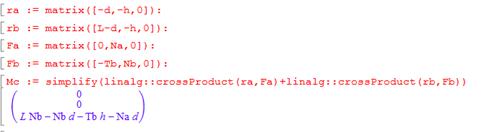
). It is essential to take moments about the particle
(i.e. the rider’s COM).
gives
It’s very simple to do the moment calculation by hand, but for those of you who find such calculations unbearable here’s a Mupad script to do it. The script simply writes out the position vectors of points A and B relative to the center of mass as 3D vectors, writes down the reactions at A and B as 3D vectors, and calculates the resultant moment (we don’t bother including the weight, because it acts at the origin and so exerts zero moment)
The two nonzero components
of and the one nonzero component of
give us three scalar equations
We
have four unknowns the reaction components
and the acceleration a so we need another equation.
The missing equation is the friction
law
5. Solution: Here’s the solution with Mupad. It’s easy to get the same answer by hand as well.
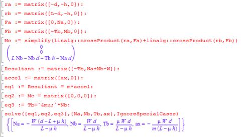
We are interested in finding what makes the reaction force at A go to zero (that’s when the bike is about to tip). So
 This tells us that the bike will tip if the friction
coefficient exceeds a critical magnitude, which depends on the geometry of the
bike. The simplest way to design a
tip-resistant bike is to make the height of the center of mass h small, and the distance (L-d) between the front wheel and the COM
as large as possible.
This tells us that the bike will tip if the friction
coefficient exceeds a critical magnitude, which depends on the geometry of the
bike. The simplest way to design a
tip-resistant bike is to make the height of the center of mass h small, and the distance (L-d) between the front wheel and the COM
as large as possible.
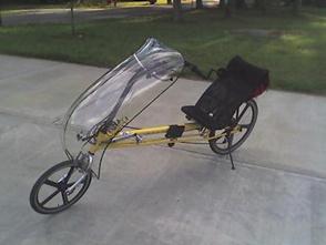
A
`recumbent’ bike is one way to achieve this the figure (from http://en.wikipedia.org/wiki/Recumbent_bicycle)
shows an example. The recumbent design offers many other significant advantages
over the classic bicycle besides tipping resistance.
 Example 4: A
stupid problem that you might find in the FE professional engineering exam. The
purpose of this problem is to show what you need to do to solve problems
involving more than one particle.
Example 4: A
stupid problem that you might find in the FE professional engineering exam. The
purpose of this problem is to show what you need to do to solve problems
involving more than one particle.
Two
weights of mass and
are connected by a cable passing over two
freely rotating pulleys as shown. They
are released, and the system begins to move.
Find an expression for the tension in the cable connecting the two
weights.
1.  Idealization
The masses will be idealized as particles; the
cable is inextensible and the mass of the pulleys is neglected. This means the internal forces in the cable,
and the forces acting between cables/pulleys must satisfy
and
,
and we can treat them as though they were in static equilibrium.
2.
FBD we have to draw a separate FBD for each
particle. Since the pulleys and cable
are massless, the tension T in the
cable is constant.
3. Kinematics We know that both masses must move in the j direction. We also know that the masses always move at the same speed but in opposite directions. Therefore, their accelerations must be equal and opposite. We can express this mathematically as
4. EOM: We must write down two equations of motion, as there are two masses
We
now have three equations for three unknowns (the unknowns are and T).
5. Solution: As paid up members of ALE (the Academy of Lazy Engineers) we use Mupad to solve the equations
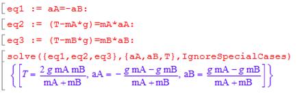
So the tension in the cable is
We pass!
 Example 5:
Another stupid FE exam problem: The figure
shows a small block on a rotating bar.
The contact between the block and the bar has friction coefficient
Example 5:
Another stupid FE exam problem: The figure
shows a small block on a rotating bar.
The contact between the block and the bar has friction coefficient . The bar rotates at constant angular speed
. Find the critical angular velocity that will
just make the block start to slip when
. Which way does the block slide?
The general approach to this
problem is the same as for the Magic trick example we will calculate the reaction force exerted
by the bar on the block, and see when the forces are large enough to cause slip
at the contact. We analyze the motion
assuming the slip does not occur, and
then find out the conditions where this can no longer be the case.
1.
 Idealization
 We will idealize the block as a particle. This is dangerous, because the block is
clearly rotating. We hope that because
it rotates at constant rate, the rotation will not have a significant effect
but we can only check this once we know how to
deal with rotational motion.
2. FBD: The figure shows a free body diagram for the block. The block is subjected to a vertical gravitational force, and reaction forces at the contact with the bar. Since we have assumed that the contact is not slipping, we can choose the direction of the tangential component of the reaction force arbitrarily. The resultant force on the block is
3. Kinematics We can use the circular motion formula to write down the acceleration of tbe block (see section 3.1.3)
4. EOM: The equation of motion is
5.
Solution: The i and j components of the equation of motion
can be solved for N and T Mupad makes this painless
To find the point where the block just starts to slip, we use the friction law. Recall that, at the point of slip
For
the block to slip with
so
the critical angular velocity is . Since the tangential traction T is negative, and the friction force
must oppose sliding, the block must
slide outwards, i.e. r is increasing
during slip.
 Alternative
method of solution using normal-tangential coordinates
Alternative
method of solution using normal-tangential coordinates
We will solve this problem again, but this time we’ll use the short-cuts described in Section 3.1.4 to write down the acceleration vector, and we’ll write down the vectors in Newton’s laws of motion in terms of the unit vectors n and t normal and tangent to the object’s path.
 (i) Acceleration vector If the block does not slip, it moves with
speed
(i) Acceleration vector If the block does not slip, it moves with
speed around a circular arc with radius r.
Its acceleration vector has magnitude
and direction parallel to the unit vector n.
(ii) The force vector can be resolved into components parallel to n and t. Simple trig on the free body diagram shows that
(iii) Newton’s laws then give
The components of this vector equation parallel to t and n yield two equations, with solution
This is the same solution as before. The short-cut makes the calculation slightly more straightforward. This is the main purpose of using normal-tangential components.
 Example 6: Window
blinds. Have you ever wondered how window shades
work? You give the shade a little
downward jerk, let it go, and it winds itself up. If you pull the shade down slowly, it stays
down.
Example 6: Window
blinds. Have you ever wondered how window shades
work? You give the shade a little
downward jerk, let it go, and it winds itself up. If you pull the shade down slowly, it stays
down.
The
figure shows the mechanism (which probably only costs a few cents to
manufacture) that achieves this remarkable feat of engineering. It’s called an `inertial latch’ the same principle is used in the inertia
reels on the seatbelts in your car.
The picture shows an enlarged end view of the window shade. The hub, shown in brown, is fixed to the bracket supporting the shade and cannot rotate. The drum, shown in peach, rotates as the shade is pulled up or down. The drum is attached to a torsional spring, which tends to cause the drum to rotate counterclockwise, so winding up the shade. The rotation is prevented by the small dogs, shown in red, which engage with the teeth on the hub. You can pull the shade downwards freely, since the dogs allow the drum to rotate counterclockwise.
To raise the shade, you need to give the end of the shade a jerk downwards, and then release it. When the drum rotates sufficiently quickly (we will calculate how quickly shortly) the dogs open up, as shown on the right. They remain open until the drum slows down, at which point the topmost dog drops and engages with the teeth on the hub, thereby locking up the shade once more.
We will estimate the critical rotation rate required to free the rotating drum.
1.
 Idealization
 We will idealize the topmost dog as a particle
on the end of a massless, inextensible rod, as shown in the figure.
a.
We will assume that the drum rotates at
constant angular rate . Our goal is to calculate the critical speed
where the dog is just on the point of dropping down to engage with the hub.
b.
When the drum spins
fast, the particle is contacts the outer rim of the drum a normal force acts at the contact. When the dog is on the point of dropping this
contact force goes to zero. So our goal
is to calculate the contact force, and then to find the critical rotation rate
where the force will drop to zero.
c. We neglect friction.
2.
 FBD. The figure
shows a free body diagram for the particle. The particle is subjected to: (i) a
reaction force N where it contacts
the rim; (ii) a tension T in the
link, and (iii) gravity. The resultant
force is
FBD. The figure
shows a free body diagram for the particle. The particle is subjected to: (i) a
reaction force N where it contacts
the rim; (ii) a tension T in the
link, and (iii) gravity. The resultant
force is
3. Kinematics We can use the circular motion formula to write down the acceleration of the particle(see section 3.1.3)
4. EOM: The equation of motion is
5.
Solution: The i and j components of the equation of motion
can be solved for N and T Mupad makes this painless
normal reaction force is therefore
We are looking for the
point where this can first become zero or negative. Note that
at the point where
=0. The
smallest value of N therefore occurs
at this point, and has magnitude
The critical speed where N=0 follows as
Changing the angle and the radius R gives a convenient way to control the critical speed in designing
an inertial latch.
Alternative solution using polar coordinates
 We’ll
work through the same problem again, but this time handle the vectors using
polar coordinates.
We’ll
work through the same problem again, but this time handle the vectors using
polar coordinates.
1. FBD. The figure shows a free body diagram for the particle. The particle is subjected to: (i) a reaction force N where it contacts the rim; (ii) a tension T in the link, and (iii) gravity. The resultant force is
2. Kinematics The acceleration vector is now
3. EOM: The equation of motion is
4. Solution: The
components of the equation of motion can be
solved for N and T
again, we can use Mupad for this
The normal reaction force is therefore
We are looking for the
point where this can first become zero or negative. Note that
at the point where
=0. The
smallest value of N therefore occurs
at this point, and has magnitude
The critical speed where N=0 follows as
Changing the angle and the radius R gives a convenient way to control the critical speed in designing
an inertial latch.
 Example 7:
Aircraft Dynamics Aircraft performing
certain instrument approach procedures (such as holding patterns or procedure
turns) are required to make all turns at a standard rate, so that a complete
360 degree turn takes 2 minutes. All
turns must be made at constant altitude and constant speed, V.
Example 7:
Aircraft Dynamics Aircraft performing
certain instrument approach procedures (such as holding patterns or procedure
turns) are required to make all turns at a standard rate, so that a complete
360 degree turn takes 2 minutes. All
turns must be made at constant altitude and constant speed, V.
People
who design instrument approach procedures need to know the radius of the
resulting turn, to make sure the aircraft won’t hit anything. Engineers designing the aircraft are
interested in the forces needed to complete the turn specifically, the load factor, which is the ratio of the lift force on the aircraft
to its weight.
In this problem we will calculate the radius of the turn R and the bank angle required, as well as the load factor caused by the maneuver, as a function of the aircraft speed V.
Before starting the calculation, it is helpful to understand what makes an aircraft travel in a circular path. Recall that
1. If an object travels at constant speed around a circle, its acceleration vector has constant magnitude, and has direction towards the center of the circle
2. A force must act on the aircraft to produce this
acceleration i.e. the resultant force on the aircraft must
act towards the center of the circle.
The necessary force comes from the
horizontal component of the lift force
the pilot banks the wings, so that the lift
acts at an angle to the vertical.
With this insight, we expect to be able to use the equations of motion to calculate the forces.
1.
Idealization The aircraft is idealized as a particle
it’s not obvious that this is accurate,
because the aircraft clearly rotates as it travels around the curve. However, the forces we wish to calculate turn
out to be fully determined by F=ma and are not influenced by the
rotational motion.
2.
 FBD. The
figure shows a free body diagram for the aircraft. It is subjected to (i) a gravitational force
(mg); (ii) a thrust from the engines
FBD. The
figure shows a free body diagram for the aircraft. It is subjected to (i) a gravitational force
(mg); (ii) a thrust from the engines ,
(iii) a drag force
,
acting perpendicular to the direction of motion, and (iv) a lift force
,
acting perpendicular to the plane of the wings.
The resultant force is
(you may find the components of the lift force
difficult to visualize to see where these come from, note that the
lift force can be projected onto components along OR and the k direction as
. Then note that
.)
3. Kinematics
a.
The aircraft moves at
constant speed around a circle, so the angle ,
where
is the (constant)
angular speed of the line OP. Since the aircraft completes a turn in two
minutes, we know that
rad/sec
b. The position vector of the plane is
We can differentiate this expression with respect to time to find the velocity
c.
The magnitude of
the velocity is ,
so if the aircraft flies at speed V,
the radius of the turn must be
d. Differentiating the velocity gives the acceleration
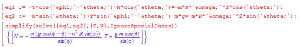
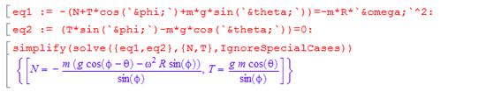
4. EOM: The equation of motion is
5.
Solution: The i j and k components of the equation of motion give three equations that
can be solved for ,
and
. We assume that the drag force is known, since
this is a function of the aircraft’s speed.
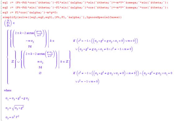
This solution is correct, but you need a PhD to understand what it means (other symbolic manipulation programs like Maple and Mathematica give a comprehensible solution). Fortunately, I happen to have a PhD… The solution can be simplified to
As we will see below, if you choose to solve this problem in normal-tangential coordinates, you don’t need a PhD to
We can calculate values of ,
and the load factor
for a few aircraft
a.
Cessna 150 V=70knots
(36 m/s) :
R=690m,
b.
Boeing 747: V=200
knots (102 m/s) R=1950m,
c.
F111 V=300 knots (154 m/s) R=2950m,
 Alternative
solution using normal-tangential coordinates
Alternative
solution using normal-tangential coordinates
This problem can also be solved rather more quickly using normal and tangential basis vectors.
(i) Acceleration vector. The aircraft travels around a circular path at constant speed, so its acceleration is
where n is a unit vector pointing towards the center of the circle.
 (ii) Force
vector. The force vector can be written in terms of the unit vectors n,t,k as
(ii) Force
vector. The force vector can be written in terms of the unit vectors n,t,k as
(iii) Newton’s law
The
n, t and k components of
this equation give three equations that can be solved for ,
and
. This time it is easy to solve the equations
by hand…
This example again shows why
normal-tangential coordinates are useful describing forces, and solving the resulting
force-acceleration relations are much simpler than working with a fixed
coordinate system.
3.3 Deriving and solving equations of motion for systems of particles
We next turn to the more difficult problem of predicting the motion of a system that is subjected to a set of forces.
3.3.1 General procedure for deriving and solving equations of motion for systems of particles
It is very straightforward to analyze the motion of systems of particles. You should always use the following procedure
1. Introduce a set of variables
that can describe the motion of the system.
Don’t worry if this sounds vague it will be clear what this means when we solve
specific examples.
2. Write down the position vector of each particle in the system in terms of these variables
3. Differentiate the position vector(s), to calculate the velocity and acceleration of each particle in terms of your variables;
4. Draw a free body diagram showing the forces acting on each particle. You may need to introduce variables to describe reaction forces. Write down the resultant force vector.
5. Write down for each particle. This will generate up to 3 equations of motion
(one for each vector component) for each particle.
6. If you wish, you can eliminate
any unknown reaction forces from you can have MATLAB calculate the reactions
for you. The result will be a set of differential equations for the variables
defined in step (1)
7. If you find you have fewer equations than unknown variables, you should look for any constraints that restrict the motion of the particles. The constraints must be expressed in terms of the unknown accelerations.
8. Identify the initial conditions for the variables defined in (1). These are usually the values of the unknown variables, their time derivatives, at time t=0. If you happen to know the values of the variables at some other instant in time, you can use that too. If you don’t know their values at all, you should just introduce new (unknown) variables to denote the initial conditions.
9. Solve the differential equations, subject to the initial conditions.
Steps (3) (6) and (8) can usually be done on the computer, so you don’t actually have to do much calculus or math.
Sometimes, you can avoid solving the equations of
motion completely, by using conservation
laws conservation of energy, or conservation of
momentum
to calculate quantities of interest. These short-cuts will be discussed in the
next chapter.
3.2.2 Simple examples of equations of motion and their solutions
The general process described in the preceding section can be illustrated using simple examples. In this section, we derive equations of motion for a number of simple systems, and find their solutions.
The purpose of these examples is to illustrate the straightforward, step-by-step procedure for analyzing motion in a system. Although we solve several problems of practical interest, we will simply set up and solve the equations of motion with some arbitrary values for system parameter, and won’t attempt to explore their behavior in detail. More detailed discussions of the behavior of dynamical systems will follow in later chapters.
Example 1: Trajectory of a particle near the earth’s surface (no air resistance)
At time t=0,
a projectile with mass m is launched from a position with
initial velocity vector
. Calculate its trajectory as a function of
time.
1.
Introduce variables to describe the
motion: We can simply use the Cartesian coordinates of the
particle
2. Write down the position vector in
terms of these variables:
3. Differentiate the position vector with respect to time to find the acceleration. For this example, this is trivial
4.
Draw a free body diagram. The only force acting on the particle is
gravity the free body diagram is shown in the figure. The force vector follows as
.
5.
Write down
The vector equation actually represents three separate differential equations of motion
6.
Eliminate reactions this is not needed in this example.
7.
Identify initial conditions. The initial conditions were given in this
problem we have that
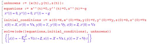
8. Solve the equations of motion. In general we will use MAPLE or matlab to do the rather tedious algebra necessary to solve the equations of motion. Here, however, we will integrate the equations by hand, just to show that there is no magic in MAPLE.
The equations of motion are
It is a bit easier to see how to solve these if we define
The equation of motion can
be re-written in terms of as
We can separate variables and integrate, using the initial conditions as limits of integration
Now we can re-write the velocity components in terms of (x,y,z) as
Again, we can separate variables and integrate
so the position and velocity vectors are
Here’s how to integrate the equations of motion using Mupad
Applications of trajectory problems: It is traditional in elementary physics and dynamics courses to solve vast numbers of problems involving particle trajectories. These invariably involve being given some information about the trajectory, which you must then use to work out something else. These problems are all somewhat tedious, but we will show a couple of examples to uphold the fine traditions of a 19th century education.
 Estimate how far you could throw a stone from
the top of the Kremlin palace.
Estimate how far you could throw a stone from
the top of the Kremlin palace.
Note that
1. The horizontal and vertical components of velocity at time t=0 follow as
2.
The components of
the position of the particle at time t=0
are
3. The trajectory of the particle follows as
4.
When the particle
hits the ground, its position vector is . This must be on the trajectory, so
where
is the time of impact.
5.
The two
components of this vector equation gives us two equations for the two unknowns ,
which can be solved
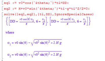
The RootOf in MAPLE is
scary any time that MAPLE gives you a scary result,
look in the help and see if there is a `convert’ function that might make it
less scary.
For a rough estimate of the distance we can use the following numbers
1.
Height of Kremlin
palace 71m
2. Throwing velocity maybe 25mph?
(pretty pathetic, I know - you can probably do better, especially if you
are on the baseball team).
3.
Throwing angle 45 degrees.
Substituting numbers gives 36m (118ft).
If you want to go wild, you
can maximize D with respect to ,
but this won’t improve your estimate much.
 Silicon nanoparticles with radius 20nm are in thermal motion near a flat
surface. At the surface, they have an
average velocity
Silicon nanoparticles with radius 20nm are in thermal motion near a flat
surface. At the surface, they have an
average velocity ,
where m is their mass, T is the
temperature and k=1.3806503 × 10⁻²³ is
the Boltzmann constant. Estimate the maximum height above the surface that a
typical particle can reach during its thermal motion, assuming that the only
force acting on the particles is gravity
1. The particle will reach its maximum height if it happens to be traveling vertically, and does not collide with any other particles.
2.
At time t=0 such a particle has position and velocity
3. For time t>0 the position vector of the particle follows as
Its velocity is
4. When the particle reaches its maximum height, its
velocity must be equal to zero (if you don’t see this by visualizing the motion
of the particle, you can use the mathematical statement that if is a maximum, then
).
Therefore, at the instant of maximum height
5.
This shows
that the instant of max height occurs at time
6. Substituting this time back into the position vector shows that the position vector at max height is
7. Si has a density of about 2330 kg/m^3. At room
temperature (293K) we find that the distance is surprisingly large: 10mm or
so. Gravity is a very weak force at the nano-scale
surface forces acting between the particles,
and the particles and the surface, are much larger.
Example 2: Free vibration of a suspension system.
A
vehicle suspension can be idealized as a mass m supported by a spring. The
spring has stiffness k and
un-stretched length . To test the suspension, the vehicle is
constrained to move vertically, as shown in the figure. It is set in motion by
stretching the spring to a length
and then releasing it (from rest). Find an expression for the motion of the
vehicle after it is released.
As
an aside, it is worth noting that a particle idealization is usually too crude
to model a vehicle a rigid body approximation is much
better. In this case, however, we assume
that the vehicle does not rotate. Under these conditions the equations of
motion for a rigid body reduce to
and
,
and we shall find that we can analyze the system as if it were a particle.
1. Introduce
variables to describe the motion: The length of the spring is a
convenient way to describe motion.
2. Write down the position vector in terms of these variables: We can take the origin at O as shown in the figure. The position vector of the center of mass of the block is then
3. Differentiate the position vector with respect to time to find the acceleration. For this example, this is trivial
 4. Draw a free body diagram.
The free body diagram is shown in the figure: the mass is subjected to
the following forces
4. Draw a free body diagram.
The free body diagram is shown in the figure: the mass is subjected to
the following forces
· Gravity, acting at the center of mass of the vehicle
· The force due to the spring
· Reaction forces at each of the rollers that force the vehicle to move vertically.
Recall the spring force law, which says that the forces exerted by a spring act parallel to its length, tend to shorten the spring, and are proportional to the difference between the length of the spring and its un-stretched length.
5.
Write down
The i and j components give two scalar equations of motion
6.
Eliminate reactions this is not needed in this example.
7.
Identify initial conditions. The initial conditions were given in this
problem at time t=0,
we know that
and
8. Solve the equations of motion. Again, we will first integrate the equations of motion by hand, and then repeat the calculation with MAPLE. The equation of motion is
We can re-write this in terms of
This gives
We can separate variables and integrate
Don’t worry if the last
line looks mysterious writing the solution in this form just makes
the algebra a bit simpler. We can now
integrate the velocity to find x
The integral on the left can be evaluated using the substitution
so that
Here’s the MAPLE solution
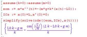
Note that it’s important to include the assume() statements, otherwise Mupad gives the solution in the form of an exponential of a complex number. The solution in this other form is also correct, but is difficult to visualize.
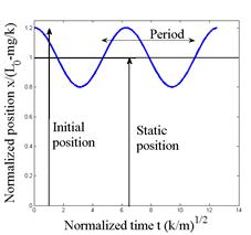 The solution is plotted in the figure. The behavior of vibrating systems will be
discussed in more detail later in this course, but it is worth noting some
features of the solution:
The solution is plotted in the figure. The behavior of vibrating systems will be
discussed in more detail later in this course, but it is worth noting some
features of the solution:
1. The average position of the mass is .
Here, mg/k is the static deflection
of the spring i.e. the deflection of the spring due to the weight of the
vehicle (without motion). This means that the car vibrates symmetrically about
its static deflection.
2.
The amplitude of vibration is . This corresponds to the distance of the mass
above its average position at time t=0.
3.
The period of oscillation (the time taken
for one complete cycle of vibration) is
4.
The frequency of oscillation (the number of cycles
per second) is (note f=1/T). Frequency is also sometimes quoted as angular frequency, which is related to f by
. Angular frequency is in radians per second.
An
interesting feature of these results is that the static deflection is related
to the frequency of oscillation - so if you measure the static deflection ,
you can calculate the (angular) vibration frequency as
Example 3: Silly FE exam problem
 This example shows how polar
coordinates can be used to analyze motion.
This example shows how polar
coordinates can be used to analyze motion.
The rod shown in the picture rotates at constant
angular speed in the horizontal plane.
The interface between block and rod has friction coefficient . The rod pushes a block of mass m, which starts at r=0 with radial speed V. Find an expression for r(t).
1. Introduce variables to describe the motion the polar coordinates
work for this problem
2. Write down the position vector and differentiate to
find acceleration we don’t need to do this
we can just write down the standard result for
polar coordinates
3. Draw a free body diagram shown in the figure
note that it is important to draw the friction
force in the correct direction. The
block will slide radially outwards, and friction opposes the slip.
4. Write down Newton’s law
5. Eliminate reactions
F=ma gives two
equations for N and T.
A third one comes from the friction law
The third solution can be rearranged into an equation of motion for r
6. Identify initial conditions Here, r=0 dr/dt=V at time t=0.
7. Solve the equation: If you’ve taken AM33 you will know how to solve this equation… But if not, or you are lazy, you can use MAPLE to solve it for you.
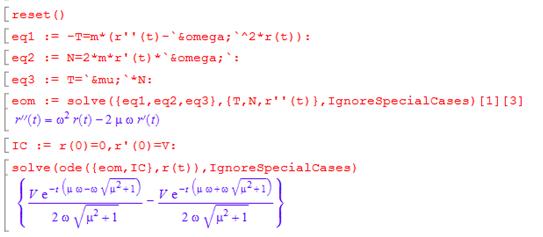
This can be simplified slightly by hand:
 Example 4: Motion of a pendulum (R-rated version)
A pendulum is a ubiquitous engineering system. You are, of course, familiar with how a pendulum can be used to measure time. But it’s used for a variety of other scientific applications. For example, Professor Crisco’s lab uses pendulum to measure properties of human joints, see
Crisco Joseph J; Fujita Lindsey; Spenciner David B, ‘The dynamic flexion/extension properties of the lumbar spine in vitro using a novel pendulum system.’ Journal of biomechanics 2007;40(12):2767-73
In this example, we will work through the basic problem of deriving and solving the equations of motion for a pendulum, neglecting air resistance.
1.
Introduce variables to describe
motion: The angle shown in the figure is a convenient variable.
2. Write down the position vector as a function of the variables We introduce a Cartesian coordinate system with origin at O, as shown in the picture.
Elementary geometry shows
that
Note
that we have assumed that the cable remains straight this will be true as long as the internal
force in the cable is tensile. If
calculations predict that the internal force is compressive, this assumption is
wrong. But there is no way to check the
assumption at this point so we simply proceed, and check the answer at the end
3. Differentiate the position vector to find the acceleration: The computer makes this painless.
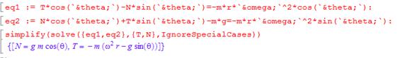
4. The free body diagram is shown in the figure. The force exerted by the cable on the particle is introduced as an unknown reaction force. The force vector is
5.
Equating the i and j components gives two equations for the two unknowns
6.
Eliminate
the reaction forces. In this problem, it is helpful to eliminate
the unknown reaction force R. You can do this on the computer if you like,
but in this case it is simpler to do this by hand. You can simply multiply the first equation by
and the second equation by
and then add them. This yields
7.
Identify
initial conditions. Some calculations are necessary to determine the
initial conditions in this problem. We
are given that at time t=0,
and the horizontal velocity is
at time t=0,
but to solve the equation of motion, we need the value of
. We can find the relationship we need by
differentiating the position vector to find the velocity
Setting and
at t=0
shows that
so
8.
Solve
the equations of motion This equation
of motion is too difficult for MAPLE but actually the solution does exist and
is very well known this is a classic problem in mathematical
physics. With initial conditions
the solution is
The first solution describes swinging motion of the pendulum, while the second solution describes the motion that occurs if you push the pendulum so hard that it whirls around on the pivot. The equations may look scary, but you can simply use MAPLE to calculate and plot them.
- In the first equation,
is a special function called the `sin amplitude.’ You can think of it as a sort of trig function for adultsin fact for k=0,and we recover the PG version. You can compute it in Mupad using jacobiSN(x,k)
- Similarly, is a function called the `Amplitude.’ You can calculate it in Mupad using jacobiAM(x,k). In Mupad, the am function has range, so the solution predicts that as the pendulum whirls around the pivot, the angleincreases from 0 to, then jumps to, increases toagain, and so on.
You
might have solved the pendulum problem already in an elementary physics course,
and might remember a different solution.
This is because you probably only derived an approximate solution, by assuming that the angle remains small. This occurs when the initial velocity
satisfies
, in which case the solution can be approximated by
3.3.3 Numerical solutions to equations of motion using MATLAB
In the preceding section, we were able to solve all
our equations of motion exactly, and hence to find formulas that describe the motion of the system. This should give you a warm and fuzzy feeling
it appears that with very little work, you can
predict everything about the motion of the system. You may even have visions of running a
consulting business from your yacht in the
Unfortunately real life is not so simple. Equations of motion for most engineering systems cannot be solved exactly. Even very simple problems, such as calculating the effects of air resistance on the trajectory of a particle, cannot be solved exactly.
For
nearly all practical problems, the equations of motion need to be solved numerically, by using a computer to
calculate values for the position, velocity and acceleration of the system as
functions of time. Vast numbers of computer programs have been written for this
purpose some focus on very specialized applications,
such as calculating orbits for spacecraft (STK); calculating motion of atoms in
a material (LAMMPS); solving fluid flow problems (e.g. fluent, CFDRC); or
analyzing deformation in solids (e.g. ABAQUS, ANSYS, NASTRAN, DYNA); others are
more general purpose equation solving programs.
In this course we will use MATLAB, which is widely used in all engineering applications. You should complete the MATLAB tutorial before proceeding any further.
In the remainder of this section, we provide a number of examples that illustrate how MATLAB can be used to solve dynamics problems. Each example illustrates one or more important technique for setting up or solving equations of motion.
Example 1: Trajectory of a particle near the earth’s surface (with air resistance)
 As a simple example we set
up MATLAB to solve the particle trajectory problem discussed in the preceding
section. We will extend the calculation
to account for the effects of air resistance, however. We will assume that our projectile is
spherical, with diameter D, and we
will assume that there is no wind. You
may find it helpful to review the discussion of aerodynamic drag forces in
Section 2.1.7 before proceeding with this example.
As a simple example we set
up MATLAB to solve the particle trajectory problem discussed in the preceding
section. We will extend the calculation
to account for the effects of air resistance, however. We will assume that our projectile is
spherical, with diameter D, and we
will assume that there is no wind. You
may find it helpful to review the discussion of aerodynamic drag forces in
Section 2.1.7 before proceeding with this example.
1. Introduce
variables to describe the motion: We can simply use the Cartesian
coordinates of the particle
2. Write down the position vector in
terms of these variables:
3. Differentiate the position vector with respect to time to find the acceleration. Simple calculus gives
4. Draw a free body diagram. The particle is now subjected to two forces, as shown in the picture.
Gravity
as always we have
.
Air resistance.
The
magnitude of the air drag force is given
by ,
where
·
is the air density,
·
is the drag coefficient,
· D is the projectile’s diameter, and
·
is the magnitude of the projectile’s velocity
relative to the air. Since we assumed the air is stationary, V is simply the magnitude of the
particle’s velocity, i.e.
The Direction
of the air drag force is always opposite to the direction of motion of the
projectile through the air. In this case
the air is stationary, so the drag force is simply opposite to the direction of
the particle’s velocity. Note that is a unit vector parallel to the particle’s
velocity. The drag force vector is
therefore
The total force vector is therefore
5.
Write down
It is helpful to simplify
the equation by defining a specific drag
coefficient ,
so that
The vector equation actually represents three separate differential equations of motion
6.
Eliminate reactions this is not needed in this example.
7. Identify initial conditions. The initial conditions were given in this problem - we have that
8. Solve
the equations of motion. We
can’t use the magic ‘dsolve’ command in MAPLE to solve this equation it has no known exact solution. So instead, we use MATLAB to generate a
numerical solution.
This takes two steps. First, we must turn the equations of motion
into a form that MATLAB can use. This
means we must convert the equations into first-order vector valued differential
equation of the general form . Then, we must write a MATLAB script to
integrate the equations of motion.
Converting the equations of motion: We can’t
solve directly for (x,y,z), because
these variables get differentiated more than once with respect to time. To fix this, we introduce the time derivatives of (x,y,z) as new unknown variables. In other words, we will solve for ,
where
These definitions are three new equations of motion relating our unknown variables. In addition, we can re-write our original equations of motion as
So, expressed as a vector valued differential equation, our equations of motion are
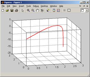
MATLAB script. The procedure for solving these equations is discussed in the MATLAB tutorial. A basic MATLAB script is listed below.
function trajectory_3d
% Function to plot trajectory of a projectile
% launched from position X0 with velocity V0
% with specific air drag coefficient c
% stop_time specifies the end of the calculation
g = 9.81; % gravitational accel
c=0.5; % The constant c
X0=0; Y0=0; Z0=0; % The initial position
VX0=10; VY0=10; VZ0=20;
stop_time = 5;
initial_w = [X0,Y0,Z0,VX0,VY0,VZ0]; % The solution at t=0
[times,sols] = ode45(@eom,[0,stop_time],initial_w);
plot3(sols(:,1),sols(:,2),sols(:,3)) % Plot the trajectory
function dwdt = eom(t,w)
% Variables stored as follows w = [x,y,z,vx,vy,vz]
% i.e. x = w(1), y=w(2), z=w(3), etc
x = w(1); y=w(2); z=w(3);
vx = w(4); vy = w(5); vz = w(6);
vmag = sqrt(vx^2+vy^2+vz^2);
dxdt = vx; dydt = vy; dzdt = vz;
dvxdt = -c*vmag*vx;
dvydt = -c*vmag*vy;
dvzdt = -c*vmag*vz-g;
dwdt = [dxdt;dydt;dzdt;dvxdt;dvydt;dvzdt];
end
end
This produces a plot that looks like this (the plot’s been edited to add the grid,etc)
 Example 2:
Simple satellite orbit calculation
Example 2:
Simple satellite orbit calculation
The figure shows satellite with mass m orbiting a planet with mass M.
At time t=0 the satellite has
position vector and velocity vector
. The planet’s motion may be neglected (this is
accurate as long as M>>m). Calculate
and plot the orbit of the satellite.
1. Introduce variables to describe the motion: We will use the (x,y) coordinates of the satellite.
2. Write down the position vector in
terms of these variables:
3. Differentiate the position vector with respect to time to find the acceleration.
4. Draw a free body diagram. The satellite is subjected to a gravitational force.
The
magnitude of the force is ,
where
·
is the gravitational constant, and
·
is the distance between the planet and the
satellite
The
direction of the force is always towards the origin: is
therefore a unit vector parallel to the direction of the force. The total force acting on the satellite is
therefore
5.
Write down
The vector equation represents two separate differential equations of motion
6.
Eliminate reactions this is not needed in this example.
7. Identify initial conditions. The initial conditions were given in this problem - we have that
8. Solve the equations of motion. We follow the usual procedure: (i) convert the equations into MATLAB form; and (ii) code a MATLAB script to solve them.
Converting the equations of motion: We introduce
the time derivatives of (x,y) as new
unknown variables. In other words, we
will solve for ,
where
These definitions are new equations of motion relating our unknown variables. In addition, we can re-write our original equations of motion as
So, expressed as a vector valued differential equation, our equations of motion are
Matlab script: Here’s a simple script to solve these equations.
function satellite_orbit
% Function to plot orbit of a satellite
% launched from position (R,0) with velocity (0,V)
GM=1;
R=1;
V=1;
Time=100;
w0 = [R,0,0,V]; % Initial conditions
[t_values,w_values] = ode45(@odefunc,[0,time],w0);
plot(w_values(:,1),w_values(:,2))
function dwdt = odefunc(t,w)
x=w(1);
y=w(2); vx=w(3); vy=w(4);
r = sqrt(x^2+y^2);
dwdt = [vx;vy;-GM*x/r^3;-GM*y/r^3];
end
end
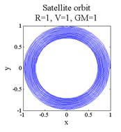
Running the script produces the result shown (the plot was annotated by hand)
Do we believe this result? It is a bit surprising the satellite seems to be spiraling in towards
the planet. Most satellites don’t do
this
so the result is a bit suspicious. The First Law of Scientific Computing states
that ` if a computer simulation predicts
a result that surprises you, it is probably wrong.’
So how can we test our computation? There are two good tests:
1. Look for any features in the simulation that you can predict without computation, and compare your predictions with those of the computer.
2. Try to find a special choice of system parameters for which you can derive an exact solution to your problem, and compare your result with the computer
We can use both these checks here.
1.
Conserved quantities For this particular problem, we
know that (i) the total energy of the system should be constant; and (ii) the
angular momentum of the system about the planet should be constant (these
conservation laws will be discussed in the next chapter for now, just take this as given). The total energy of the system consists of
the potential energy and kinetic energy of the satellite, and can be calculated
from the formula
The total angular momentum of the satellite (about the origin) can be calculated from the formula
(If you don’t know these formulas, don’t
panic we will discuss energy and angular momentum in
the next part of the course)
We
can have MATLAB plot E/m and ,
and see if these are really conserved. The energy and momentum can be calculated by
adding these lines to the MATLAB script
for i =1:length(t)
r = sqrt(w_values(i,1)^2 + w_values(i,2)^2)
vmag = sqrt(w_values(i,1)^2 + w_values(i,2)^2)
energy(i) = -GM/r + vmag^2/2;
angularm(i) = w_values(i,1)*w_values(i,4)-w_values(i,2)*w_values(i,3);
end
You can then plot the results (e.g. plot(t_values,energy)). The results are shown below.
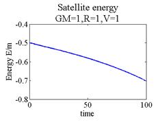
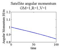
These
results look really bad neither energy, nor angular momentum, are
conserved in the simulation. Something
is clearly very badly wrong.
 Comparison to exact solution: It is not always possible to
find a convenient exact solution, but in this case, we might guess that some
special initial conditions could set the satellite moving on a circular path. A circular path might be simple enough to
analyze by hand. So let’s assume that
the path is circular, and try to find the necessary initial conditions. If you
still remember the circular motion formulas, you could use them to do
this. But only morons use formulas
Comparison to exact solution: It is not always possible to
find a convenient exact solution, but in this case, we might guess that some
special initial conditions could set the satellite moving on a circular path. A circular path might be simple enough to
analyze by hand. So let’s assume that
the path is circular, and try to find the necessary initial conditions. If you
still remember the circular motion formulas, you could use them to do
this. But only morons use formulas here we will derive the solution from scratch.
Note that, for a circular path
(a) the particle’s radius r=constant. In fact, we know r=R, from the position at time t=0.
(b) The satellite must move
at constant speed, and the angle must increase linearly with time, i.e.
where
is a constant (see section 3.1.3 to review
motion at constant speed around a circle).
With this information we can solve the equations of motion. Recall that the position, velocity and acceleration vectors for a particle traveling at constant speed around a circle are
We
know that from the initial conditions, and
is constant. This tells us that
Finally, we can substitute
this into
Both components of the equation of motion are satisfied if we choose
So, if we choose initial
values of satisfying this equation, the orbit will be
circular. In fact, our original choice,
should have given a circular orbit. It did not.
Again, this means our computer generated solution is totally wrong.
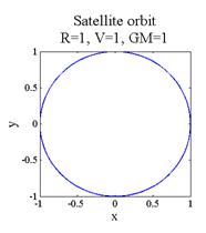 Fixing the
problem: In general, when computer predictions are
suspect, we need to check the following
Fixing the
problem: In general, when computer predictions are
suspect, we need to check the following
1. Is there an error in our MATLAB program? This is nearly always the cause of the problem. In this case, however, the program is correct (it’s too simple to get wrong, even for me).
2. There may be something wrong with our equations of motion (because we made a mistake in the derivation). This would not explain the discrepancy between the circular orbit we predict and the simulation, since we used the same equations in both cases.
3. Is the MATLAB solution sufficiently accurate? Remember that by default the ODE solver tries to give a solution that has 0.1% error. This may not be good enough. So we can try solving the problem again, but with better accuracy. We can do this by modifying the MATLAB call to the equation solver as follows
options = odeset('RelTol',0.00001);
[t_values,w_vlues] = ode45(@odefunc,[0,time],w0,options);
- Is there some feature of the equation of motion that makes them especially difficult to solve? In this case we might have to try a different equation solver, or try a different way to set up the problem.
The figure on the right shows the orbit predicted
with the better accuracy. You can see
there is no longer any problem the orbit is perfectly circular. The figures below plot the energy and
angular momentum predicted by the computer.
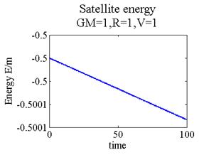
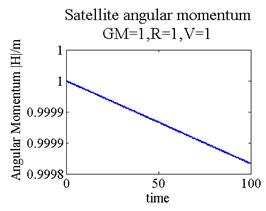
There is a small change in energy and angular momentum but the rate of change has been reduced dramatically. We can make the error smaller still by using improving the tolerances further, if this is needed. But the changes in energy and angular momentum are only of order 0.01% over a large number of orbits: this would be sufficiently accurate for most practical applications.
Most ODE
solvers are purposely designed to lose a small amount of energy as the
simulation proceeds, because this helps to make them more stable. But in some applications this is unacceptable
for example in a molecular dynamic simulation
where we are trying to predict the entropic response of a polymer, or a free
vibration problem where we need to run the simulation for an extended period of
time. There are special ODE solvers that
will conserve energy exactly.
Example 3: Earthquake response of a 2-storey building
 The figure shows a very
simple idealization of a 2-storey building.
The roof and second floor are idealized as blocks with mass m.
They are supported by structural columns, which can be idealized as
springs with stiffness k and
unstretched length L. At time t=0
the floors are at rest and the columns have lengths
The figure shows a very
simple idealization of a 2-storey building.
The roof and second floor are idealized as blocks with mass m.
They are supported by structural columns, which can be idealized as
springs with stiffness k and
unstretched length L. At time t=0
the floors are at rest and the columns have lengths (can you show this?). We will neglect the thickness of the floors
themselves, to keep things simple.
For
time t>0, an earthquake makes the
ground vibrate vertically. The ground motion can be described using the
equation . Horizontal motion may be neglected. Our goal
is to calculate the motion of the first and second floor of the building.
It is worth noting a few points about this problem:
1. You may be skeptical that the floor of a building can
be idealized as a particle (then again, maybe you couldn’t care less…). If so, you are right it certainly is not a `small’ object. However, because the floors move vertically
without rotation, the rigid body equations of motion simply reduce to
and M=0,
where the moments are taken about the center of mass of the block. The floors behave as though they are
particles, even though they are very large.
2. Real earthquakes involve predominantly horizontal, not vertical motion of the ground. In addition, structural columns resist extensional loading much more strongly than transverse loading. So we should really be analyzing horizontal motion of the building rather than vertical motion. However, the free body diagrams for horizontal motion are messy (see if you can draw them) and the equations of motion for vertical and horizontal motion turn out to be the same, so we consider vertical motion to keep things simple.
3. This problem could be solved analytically (e.g. using
the `dsolve’ feature of MAPLE) a numerical solution is not necessary. Try this for yourself.
1. Introduce
variables to describe the motion: We will use the height of each floor as the variables.
2. Write down the position vector in terms of these variables: We now have to worry about two masses, and must write down the position vector of both
Note that we must measure the position of each mass from a fixed point.
3. Differentiate the position vector with respect to time to find the acceleration.
 4. Draw a free body diagram. We must draw a free body diagram for
each mass. The resultant force acting on the bottom and top masses,
respectively, are
4. Draw a free body diagram. We must draw a free body diagram for
each mass. The resultant force acting on the bottom and top masses,
respectively, are
where
are the forces in the two springs (note that
we assume that all the springs are in tension
this makes the calculation easier).
The spring forces are equal to the stiffness multiplied by the increase in length of the springs
We
will have to find the spring lengths in terms of our coordinates
to solve the problem. Geometry shows that
So, finally
5.
Write down
This is two equations of
motion we can substitute for
and rearrange them as
6.
Eliminate reactions this is not needed in this example.
7. Identify initial conditions. We know that, at time t=0
8. Solve the equations of motion. We need to (i) reduce the equations to the standard MATLAB form and (ii) write a MATLAB script to solve them.
Converting the equations. We now need
to do two things: (a) remove the second derivatives with respect to time, by
introducing new variables; and (b) rearrange the equations into the form . We remove the derivatives by introducing
as additional unknown variables, in the usual
way. Our equations of motion can then
be expressed as
We can now code MATLAB to solve these equations directly for dy/dt. A script (which plots the position of each floor as a function of time) is shown below.
function building
%
k=100;
m=1;
omega=9;
d=0.1;
L=10;
time=20;
g = 9.81;
w0 = [L-m*g/k,2*L-3*m*g/(2*k),0,0];
[t_values,w_values] = ode45(@eom,[0,time],w0);
plot(t_values,w_values(:,1:2));
function dwdt = eom(t,w)
y1=w(1);
y2=w(2);
v1=w(3);
v2=w(4);
dwdt =
[v1;v2;...
-2*k*(y1-d*sin(omega*t)-L)/m+2*k*(y2-y1-L)/m;...
-g-2*k*(y2-y1-L)/m]
end
end
The figures below plot the height of each floor as a function of time, for various earthquake frequencies. For special earthquake frequencies (near the two resonant frequencies of the structure) the building vibrations are very severe. As long as the structure is designed so that its resonant frequencies are well away from the frequency of a typical earthquake, it will be safe.
We will discuss vibrations in much more detail later in this course.
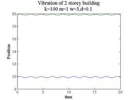
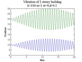
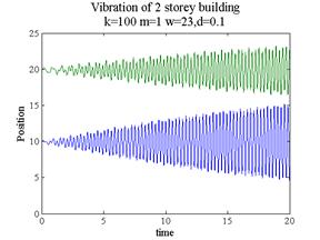
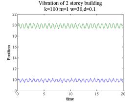
This problem illustrates a shortcoming of solving problems on the computer without thinking too much about them. The way we set up the problem, it looks as though the solution depends on g, and the unstretched spring length L, but in fact this is not the case. Not being aware of this makes the equations of motion much more complicated than they really are, and makes it harder to interpret the results. Of course we could learn by trial and error that the solution is independent of L and g, but a better approach is to eliminate these variables from the equations of motion altogether.
There is a standard way to do this instead of solving for the lengths of the
springs y, we solve for the deflection of the masses from their static
equilibrium positions. We
will discuss this in more general terms when we discuss vibration problems
later in the course. But we’ll work
through the process here, because it’s useful to use the same approach in the
mass launcher design project.
 The figure illustrates the
idea. The figure on the left shows the
masses at their static equilibrium positions. Here the springs have lengths
The figure illustrates the
idea. The figure on the left shows the
masses at their static equilibrium positions. Here the springs have lengths . We are now going to describe the motion by
the displacement of each mass from its static equilibrium position,
. We simply work through the derivations again
with these new variables.
The accelerations of the masses don’t depend on what we use for the origin (provided the origin is fixed, of course), so
The free body diagram doesn’t change either, and the forces in the springs are still given by
But
now we have to find the spring lengths in terms of our coordinates
to solve the problem. Geometry shows that
Newton’s laws of motion now become
Finally substituting for and simplifying we find that lots of terms
magically cancel, and
These equations don’t involve L or g. Furthermore the initial conditions are simply
so
the solution for must be independent of L and g.
 Example 4:
The dreaded pendulum revisited (apologies…)
Example 4:
The dreaded pendulum revisited (apologies…)
You may have lost interest in pendulum problems by now. Bear with us, however- it is a convenient example that illustrates how to solve problems with constraints.
So we re-visit the problem shown in the figure. This time, we will describe the system using (x,y) coordinates of the mass instead of the inclination of the cable.
1. Introduce
variables to describe the motion: We will use the position of the mouse
relative to point O as the variables.
2. Write down the position vector in terms of these variables:
Note that we’ve chosen j to point vertically downwards
3. Differentiate the position vector with respect to time to find the acceleration.
4.
Draw a free body diagram. We
can use the FBD we drew earlier. The
force must now be expressed in terms of x
and y instead of ,
however. Simple trig shows that
The resultant force is therefore
5.
Write down
This is two equations of
motion we can rearrange them as
6. Eliminate
reactions We
could eliminate R if we wanted
but this time we won’t bother. Instead, we will carry R along as an additional unknown, and use MATLAB to calculate
it.
7.
If
there are more unknown variables than equations of motion, look for constraint
equations. We now have three unknowns (x,y,R) but only two equations of motion
(eliminating R in step 6 won’t help in this case we will have two unknowns but
only one equation of motion). So we need
to look for an additional equation somewhere.
The
reason we’re missing an equation is that we took x,y to be arbitrary but of course the mouse has to remain attached
to the cable at all times. This means
that his distance from O is fixed
i.e.
This is the missing equation.
We could, if we wanted, use this equation to eliminate one of our unknown variables (doing the algebra by hand). Instead, however, we will use MATLAB to do this for us. For this purpose, we need to turn the equation into a constraint on the accelerations, instead of the position of the particle. To get such an equation, we can differentiate both sides of the constraint with respect to time
This is now a constraint on the velocity. Differentiating again gives
Again
if you have trouble doing the derivatives,
just use MAPLE (don’t forget to specify that x, y are functions of
time, i.e. enter them as x(t), y(t) when typing the constraint formula into
MAPLE).
[Aside when
I first coded this problem I tried to constrain the velocity of the particle, instead of the acceleration. This doesn’t work (as I should have known),
and produces some rather interesting MATLAB errors
if you are curious, try it and see what
happens. If you are even more curious,
you might like to think about why
you need to constrain accelerations and not velocities.]
7. Identify initial conditions. We know that, at time t=0
8. Solve the equations of motion. We need to (i) reduce the equations to the standard MATLAB form and (ii) write a MATLAB script to solve them.
In the usual way, we introduce as additional unknowns. Our set of unknown
variables is
. The equations of motion, together with the
constraint equation, can be expressed as
This can be expressed as a matrix equation for an unknown
vector
We
can now use MATLAB to solve the equations for the unknown time derivatives ,
together with the reaction force R. Here’s a MATLAB script that integrates the
equations of motion and plots (x,y)
as a function of time. Notice that,
because we don’t need to integrate R
with respect to time, the function ‘eom’ only needs to return
.
function pendulum
g = 9.81;
l=1;
V0=0.1;
time=20;
w0 = [0,l,V0,0]; % Initial conditions
[t_values,w_values] = ode45(@eom,[0,time],w0);
plot(t_values,w_values(:,1:2));
function dwdt = eom(t,w)
% The vector w contains [x,y,vx,vy]
x=w(1);y=w(2);vx=w(3);vy=w(4);
M = eye(5); % This sets up a 5x5 matrix with 1s on all the diags
M(3,5) = (x/m)/sqrt(x^2+y^2);
M(4,5) = (y/m)/sqrt(x^2+y^2);
M(5,3) = x;
M(5,4) = y;
M(5,5) = 0;
f = [vx;vy;0;g;-vx^2-vy^2];
sol = M\f; % This solves the matrix equation M*[dydt,R]=f for [dwdt,R]
dwdt = sol(1:4); % only need to return time derivatives dw/dt
end
end
Final
remarks: In
general, it is best to avoid using constraint equations it makes the problem harder to set up, and
harder for MATLAB to solve. Sometimes they are unavoidable, however
in some cases you might not see how to
identify a suitable set of independent coordinates; and there are some systems
(a rolling wheel is the most common example) for which a set of independent
coordinates do not exist. These are
given the fancy name `non-holonomic systems’
mentioning that you happen to be an expert on
non-holonomic systems during a romantic candle-light dinner is sure to impress
your dates.
3.3.4 Case Study - Simple model of a vehicle
As a representative application of the methods
outlined in the preceding section, we will set up and solve the equations of
motion for a very simple idealization of a vehicle. This happens to be an example of a non-holonomic system (sorry we aren’t at
a romantic dinner). Don’t worry if the
model looks rather scary this calculation is more advanced than
anything you would be expected to do at this stage of your career… Our goal is to illustrate how the method we’ve
developed in this section can be applied to a real engineering system of
interest. You should be able to follow and understand
the procedure.
The figure shows how the vehicle is idealized. Here are a few remarks:
1. We consider only 2D planar motion of the vehicle
2. For simplicity we assume the vehicle has only two wheels, one at the front and one at the rear. (It’s not a motorcycle, however, because we won’t account for the vehicle leaning around corners)
3. The car is idealized as a particle with mass m supported on a massless chassis with wheelbase L.
4. Aerodynamic drag forces are assumed to act directly on the particle.
5. The most complicated and important part of a vehicle dynamics model is the description of how the wheels interact with the road. Here, we will just assume that
a. The front and rear of the vehicle have to move in a direction perpendicular to each wheel’s axle. Reaction forces must act on each wheel parallel to the axle in order to enforce this constraint (see the FBD).
b. In addition, we assume that
the vehicle has rear-wheel drive. This is modeled as a prescribed force exerted by the ground on the rear wheel,
acting parallel to the rolling direction of the wheel (see the FBD).
c. The front wheel is assumed to roll freely and have
negligible mass this means that the contact force acting on
the wheel must be perpendicular to its rolling direction (see the FBD). The
vehicle is steered by rotating the front wheel through an angle
with respect to the chassis.
This is a vastly over-simplified model of wheel/road
interaction for example, it predicts that the car can
never skid. If you are interested in
extending this calculation to a more realistic model, ask us… We’d be happy to
give you better equations!
1.
Introduce variables to describe the
motion: We will use the (x,y)
coordinates of car and its orientation as the variables.
2. Write down the position vector in
terms of these variables:
3. Differentiate the position vector with respect to time to find the acceleration.
 4. Draw a free body diagram. The vehicle is subjected to (i) a
thrust force P and a lateral reaction
force
4. Draw a free body diagram. The vehicle is subjected to (i) a
thrust force P and a lateral reaction
force acting on the rear wheel, (ii) a lateral
reaction force
acting on the front wheel, and a drag force
acting at the center of mass.
The drag force is related to the vehicle’s velocity by
where c is a drag coefficient. For a more detailed discussion of drag forces see the first example in this section.
The resultant force on the vehicle is
Because we are modeling the motion of the vehicle’s chassis, which can rotate, we must also consider the moments acting on the chassis. You should be able to verify for yourself that the resultant moment of all the forces about the particle is
5.
Write down
This gives two equations of motion; the condition M=0 for the chassis gives one more.
6. Eliminate
reactions It’s easier to eliminate them with MATLAB.
7. If there are more unknown variables than equations of motion, look for constraint equations. This is the hard part of this application. We have two unknown reaction forces, so we need to find two constraint equations that will determine them. These are (i) that the rear of the vehicle must move perpendicular to the axle of the rear wheel; and (ii) the front of the vehicle must move perpendicular to the axle of the front wheel. Consider the rear wheel:
1. Note
that the position vector of the rear wheel is
2. The velocity follows as
3. Note that is a unit vector parallel to the axle of the
rear wheel.
4. For the rear of the vehicle to move perpendicular to
the rear axle, we must have .
This shows that
Similarly, for the front wheel, we can show that
where we have used the trig
formula .
We need to re-write these equations as constraints on the acceleration of the vehicle. To do this, we differentiate both constraints with respect to time, to see that
7. Identify initial conditions: We will assume that the vehicle starts at rest, with
7. Solve the equations of motion. We need to write the equations of motion in a suitable matrix form for MATLAB. We need to eliminate all the second derivatives with respect to time from the equations of motion, by introducing new variables. To do this, we define
as new variables, and then
solve for . We also need to eliminate the unknown
reactions. It is not hard to show that
the equations of motion, in matrix form, are
where
Finally,
we can type these into MATLAB here’s a simple script that solves the
equations of motion and plots the (x,y)
coordinates of the car to show its path, and also plots the speed of the car as
a function of time. The example
simulates a drunk-driver, who steers with steering angle
,
and drives with his or her foot to the floor with P=constant.
function drivemycar
L=1;
m=1;
c=0.1;
time=120;
y0 = [0,0,0,0,0,0];
options = odeset('RelTol',0.00001);
[t_vals,w_vals] = ode45(@eom,[0,time],y0,options);
plot(w_vals(:,1),w_vals(:,2));
function [alpha,dadt,P]=driver(t)
% This function behaves like the driver of the car -
% at time t it returns the steering angle alpha
% dalpha/dt and the driving force P
alpha = 0.1+0.2*sin(t);
dadt = 0.2*cos(t);
P = 0.2;
end
function dwdt = eom(t,w)
% Equations of motion for the vehicle
%
[alpha,dadt,P] = driver(t); % Find out what the driver is doing
M = zeros(8); % This sets up a 8x8 matrix full of zeros
M(1,1) = 1;
M(2,2) = 1;
M(3,3) = 1;
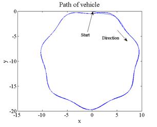 M(4,4)
= m;
M(4,4)
= m;
M(4,7)=-sin(w(3)+alpha);
M(4,8)=-sin(w(3));
M(5,5)=m;
M(5,7)=-cos(w(3)+alpha);
M(5,8)=-cos(w(3));
M(6,7)=cos(alpha);
M(6,8)=-1;
M(7,4)=sin(w(3));
M(7,5)=cos(w(3));
M(7,6)=L/2;
M(8,4)=sin(w(3)+alpha);
M(8,5)=cos(w(3)+alpha);
M(8,6)=-L*cos(alpha)/2;
v = sqrt(w(4)^2+w(5)^2);
f = [w(4);
w(5);
w(6);
P*cos(w(3))-c*v*w(4);
-P*sin(w(3))-c*v*w(5);
0;
(-cos(w(3))*w(4)+sin(w(3))*w(5))*w(6);
(-cos(w(3)+alpha)*w(4)+sin(w(3)+alpha)*w(5))*(w(6)+dadt)-sin(alpha)*L*w(6)*dadt/2];
sol = M\f; % This solves the matrix equation M*[dwdt,R]=f for [dwdt,R]
dwdt = sol(1:6); % only need to return time derivatives dw/dt
end
end
3.4 Review of concepts for Chapter 3
3.4.1 Concept checklist
Here are the skills that you should develop based on the material in this chapter:
· Be able to idealize an engineering design as a set of particles, and know when this idealization will give accurate results
· Choose an appropriate set of geometric variables to describe the motion of a system of particles (eg components in a fixed coordinate system; components in a polar coordinate system, etc)
· Be able to differentiate position vectors (with proper use of the chain rule!) to determine velocity and acceleration; and be able to integrate acceleration or velocity to determine position vector.
· Be familiar with simple harmonic motion and definitions of amplitude, frequency and period
· Be able to describe motion in normal-tangential and polar coordinates (eg be able to write down vector components of velocity and acceleration in terms of speed, radius of curvature of path, or coordinates in the cylindrical-polar system).
· Be able to convert between Cartesian to normal-tangential or polar coordinate descriptions of motion
· Be able to draw a correct free body diagram showing forces acting on system idealized as particles
· Understand and be able to describe mathematically the forces exerted by springs and dampers, and draw forces exerted by springs/dampers on a free body diagram.
· Be able to write down Newton’s laws of motion in rectangular, normal-tangential, and polar coordinate systems
· Be able to obtain an additional moment balance equation for a rigid body moving without rotation or rotating about a fixed axis at constant rate.
· Be able to use Newton’s laws of motion to solve for unknown accelerations or forces in a system of particles
· Use Newton’s laws of motion to derive differential equations governing the motion of a system of particles
· Solve the differential equations of motion analytically using Mupad, for cases where analytical solutions are available
· Be able to re-write second order differential equations as a pair of first-order differential equations in a form that MATLAB can solve
· Write a MATLAB script to solve differential equations governing the motion of a system
Of course, these are all just tricks of the trade. They are supposed to help you design a system that does something useful; or to understand (and ultimately to predict) the behavior of some physical or biological system.
3.4.2 Summary of main equations and definitions
Position-velocity-acceleration relations in a Cartesian Frame
The direction of the velocity vector is tangent to its path.
The magnitude of the velocity vector is the distance traveled along the path
per unit time (speed).
A unit vector tangent to the path can be found as
Straight line motion with constant acceleration
Here,
a is the (constant) acceleration; are the position and speed at time t=0.
Straight line motion with time/position dependent acceleration
Acceleration
given as a function of time:
Acceleration
given as a function of position
Separation of variables for one-dimensional motion
Simple Harmonic Motion 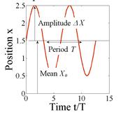
Circular Motion at Constant Speed
General Circular Motion

Note
that the straight-line motion relations can be used to relate ,
by exchanging
Motion along an arbitrary path in normal-tangential coordinates
For
a path with
Position-velocity-acceleration relations in polar-coordinates
Newton’s laws
For
a particle
For
a rigid body moving without rotation or rotating at fixed angular rate about a
fixed axis (you
must take moments about the center of mass)
Drawing free body diagrams:
1. Decide which part of a system you will idealize as a particle (you may need more than one particle)
2. Draw the part of the system you have idealized as a particle
by itself (very important!). It is important to make sure that your
particle is isolated it can’t be touching something else. You may
need more than one drawing if you have more than one particle in your system.
3. Draw on any of the following external forces that apply. Make sure you draw them acting in the correct direction, acting on the correct part of the body:
a. gravity (at the COM);
b.
air resistance or
lift forces (and sometimes moments) various conventions are used to locate these
forces but in this course we usually put them at the COM and neglect moments;
c. Buoyancy forces (act at the COM of the displaced fluid)
d. Electrostatic or electromagnetic forces
4. Draw the forces exerted by springs attached to the
particle. It is best to assume that
springs always pull on the point they are connected to, and that the magnitude
of the force in the spring is ,
where l is the length of the spring,
and
is its unstretched length.
5. Draw the forces exerted by dashpots or dampers (like
springs, assume they pull on the object they are connected to, and exert a
force magnitude where l is
the length of the dashpot.
6. Draw forces exerted by cables. Cables always pull, and exert a force parallel to the direction of the cable. The magnitude of the force has to be left as an unknown.
7. Draw any unknown reaction forces, with the following rules:
a. Reaction forces must act at any point on any point of the body that is touching something outside the particle (i.e. a part of your system that you did not include in your drawing in step 2).
b. If the connection between the two touching objects prevents them from rotating with respect to one another (or, like a motor, makes them rotate with some controllable angular speed), you will need to draw both reaction forces and moments. (Reaction moments do sometimes come up in dynamics problems, but they are not very common, so think carefully before including them).
c.
If friction acts at the contact point, and you
don’t know whether the two objects slide at the contact (or you know they do
not slide), draw both a normal and a tangential force with unknown magnitudes N,T (or some suitable variable). The direction of the friction force is not
important. DO NOT assume .
d.
If friction acts
at the contact point, and you know the contact slips, draw both a tangential and a normal
force. You must draw the tangential
force so that it opposes the direction of sliding (ask a faculty member or TA
if you don’t understand this). If slip
occurs you can assume .
e. If the contact point is frictionless, draw only a normal force.
f. If your particle is being touched by a two-force member (no, this is not a gender and sexuality class… a two force member is a massless rod, connected through freely rotating hinges at both ends. A massless freely rotating wheel can also be idealized as a two-force member) you can assume the reaction force acts parallel to the two-force member.
g. If you have more than one particle in your system, make sure that any forces exerted by one particle on the other have equal and opposite reactions.
Calculating unknown forces or accelerations using Newton’s laws:
1. Decide how to idealize the system (what are the particles?)
2. Draw a free body diagram showing the forces acting on each particle
3. Consider the kinematics
of the problem. The goal is to calculate the acceleration of each particle in
the system you may be able to start by writing down the
position vector and differentiating it, or you may be able to relate the
accelerations of two particles (eg if two particles move together, their
accelerations must be equal).
4. Write down F=ma for each particle.
5. If you are solving a problem involving a massless
frames (see, e.g. Example 3, involving a bicycle with negligible mass) you also
need to write down about the particle.
6. Solve the resulting equations for any unknown components of force or acceleration (this is just like a statics problem, except the right hand side is not zero).
Problems like this will usually ask you to make some design prediction at the end, which might involve calculating critical conditions for something to slip, tip, break, etc.
·
At the onset of
slip at a contact
· At the critical point where an object tips over, a reaction force somewhere will go to zero. You will have to identify where this point is, find the reaction force, and set it to zero.
Deriving equations of motion for a system of particles
1. Introduce a set of variables
that can describe the motion of the system.
Don’t worry if this sounds vague it will be clear what this means when we solve
specific examples.
2. Write down the position vector of each particle in the system in terms of these variables
3. Differentiate the position vector(s), to calculate the velocity and acceleration of each particle in terms of your variables;
4. Draw a free body diagram showing the forces acting on each particle. You may need to introduce variables to describe reaction forces. Write down the resultant force vector.
5. Write down for each particle. This will generate up to 3 equations of
motion (one for each vector component) for each particle.
6. If you wish, you can
eliminate any unknown reaction forces from you can have MATLAB calculate the reactions
for you. The result will be a set of differential equations for the variables
defined in step (1)
7. If you find you have fewer equations than unknown variables, you should look for any constraints that restrict the motion of the particles. The constraints must be expressed in terms of the unknown accelerations.
8. Identify the initial conditions for the variables defined in (1). These are usually the values of the unknown variables, their time derivatives, at time t=0. If you happen to know the values of the variables at some other instant in time, you can use that too. If you don’t know their values at all, you should just introduce new (unknown) variables to denote the initial conditions.
9. Solve the differential equations, subject to the initial conditions.
Trajectory equations for particle moving near earth’s surface with no air resistance
Solving differential equations with Mupad:
Example: to solve
with
initial conditions at time t=0
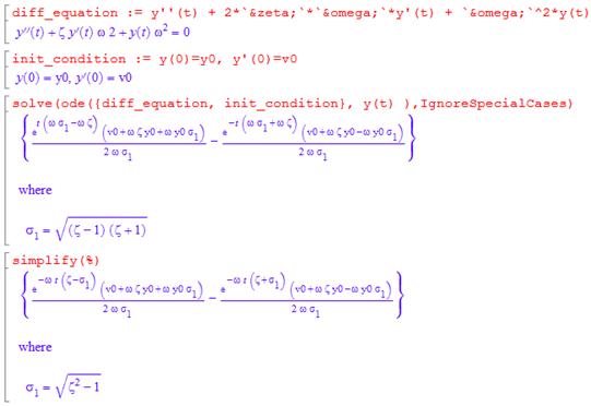
Re-writing a second-order differential equation as a pair of first-order equations for MATLAB
Example: to solve
we
introduce as an additional variable. This new equation, together with the
original ODE can then be written in the following form
This is now in the form
as required.