Chapter 6
Rigid Body Dynamics
6.1 Introduction
In practice, it is often not possible to idealize a
system as a particle. In this section,
we construct a more sophisticated description of the world, in which objects rotate, in addition to translating. This general branch of physics is called
‘Rigid Body Dynamics.’
Rigid body dynamics has many applications. In vehicle dynamics, we are often more
worried about controlling the orientation of our vehicle than its path an aircraft must keep its shiny side up, and
we don’t want a spacecraft tumbling uncontrollably. Rigid body mechanics is used extensively to
design power generation and transmission systems, from jet engines, to the
internal combustion engine, to gearboxes.
A typical problem is to convert rotational motion to linear motion, and
vice-versa. Rigid body motion is also of great interest to people who design
prosthetic devices, implants, or coach athletes: here, the goal is to understand
human motion, to protect athletes from injury or improve their performance, or
to design devices that replicate the complicated motion of a human joint
correctly. For example, Professor
Crisco’s orthopaedics lab at
Brown studies human
motion and the forces they generate at human joints, to help understand how
injuries occur and how they can be prevented.
The motion of a rigid body is often very
counter-intuitive. That’s why there are
so many toys that exploit the properties of rigid bodies: the motion of a
spinning top; a boomerang; the ‘rattleback’ and a Frisbee can all be explained
using the equations derived in this section.
Here is a quick outline of how we analyze motion of rigid bodies.
- A rigid body is idealized as an
infinite number of small particles, connected by two-force members.
- We already know the equations of
motion for a system of particles (Section 4 of the notes):
The force-momentum equation
The moment angular momentum equation
The work-kinetic energy equation
- These
equations tell us how a rigid body moves.
But to use them, we would need to keep track track of an infinite
number of particles! To simplify
the problem, we set up some mathematical methods that allow us to express
the position and velocity of every point in a rigid body in terms of the
position , velocity and acceleration of its center of mass, and its rotation
tensor R(quantifying its
orientation) and its angular velocity , and angular acceleration . This allows us to write the linear momentum,
angular momentum, and kinetic energy of a rigid body in the form
where is the total mass of the body and is its mass moment of inertia.
- We can then derive the rigid
body equations of motion:
6.2 Describing
Motion of a Rigid Body
We describe motion of a particle using its position,
velocity and acceleration. We can
describe the position of a rigid body
in the same way - we could specify the
position, velocity and acceleration of any convenient point in the body (we
usually use the center of mass). But we
also need a way to describe the orientation
of a rigid body, and its rotational motion.
 In this section, we define the various mathematical
quantities that we use to describe rotation, angular velocity, and angular
acceleration.
In this section, we define the various mathematical
quantities that we use to describe rotation, angular velocity, and angular
acceleration.
6.2.1 Describing rotations: The Rotation
Tensor (or matrix)
Rotations are quantified by a mathematical object
called a rotation tensor. It is defined as follows:
1.
Choose some
convenient initial orientation of the rigid body (eg for the rectangular prism
in the figure, we chose to make the faces perpendicular to the directions.
2.
When the body is
rotated, every line in the body (eg the sides) moves to a new orientation,
without changing its length. We can
describe this orientation change as a mapping. Let A and B be two arbitrary points in the
body. Let be the initial positions of these points, and
let be their final positions. We introduce the ‘rotation tensor’ R which has the property that
When we solve problems, we always express vectors as components in some
basis. When we do this, R becomes a matrix. For example, if
we would write
Here, are a set of nine numbers (or sometimes
formulas). Following the usual rules of
matrix-vector multiplication, this is just a short-hand notation for
The subscripts on R are meant to you help remember what
each element in the matrix does for example, maps the onto x, maps the onto x,
and so on.
So when we solve a problem, how do we go about finding R? Let me count the ways:
Rotations in two dimensions:
Life is simple in 2D.
In this case our rigid body must lie in the i,j plane, so we can only rotate it about an axis parallel to the k direction. A counter-clockwise rotation through an angle
about the k
axis is produced by
For example, a vector Li that start parallel to the i axis is mapped to
Rotation about a known axis
3D is a bit more difficult. Any
rotation can always be expressed as a rotation through some angle about some axis parallel to a unit vector n (we
always use the right hand screw convention). In some problems you can see what n and are: then you can write down a unit vector
parallel to n
and then use the ‘Rodriguez Formula’
(This formula is impossible to remember that’s what Google is for).
If you are given a rotation matrix R,
and need to find n and , you can use the formulas:
The second formula blows up if . If is zero or you can simply set (the identity), and n can be anything you like.
For you can use
The signs of the square roots have to be chosen so that
In robotics, game engines, and vehicle dynamics the
axis-angle representation of a rotation is often stored as a quaternion. We won’t use that here, but mention it in
passing in case you come across it in practice. A quaternion is four numbers that are related to n and through the formulas:
Mapping the coordinate axes
In some problems we might know what happens to vectors
that are parallel to the {i,j,k}
directions in the initial rigid body (eg we might know what happens to the
sides of our rectangular prism). For
example, we might know that map to (unit)
vectors . In
that case we can write down each of as components in
and use the formula
A sequence of rotations
Suppose we rotate an object twice (perhaps about two different
axes). How do we describe the result of
two rotations? That’s not hard. Suppose we do the first rotation with one
mapping
Now we rotate our body again this maps onto some new vector :
We can therefore write
We see that Sequential rotations
are matrix products
Health warning: Matrix products
(and hence sequences of rotations) do not commute
For example, the figure below shows the change in
orientation caused by (a) a 90 degree positive rotation about i followed by a 90 degree positive
rotation about k (the figure on the
left); and (b) a 90 degree positive rotation about k followed by a 90 degree positive rotation about i (the figure on the right).
Orthogonality of R
The rotation tensor (matrix) has a very important property:
If you
multiply R by its transpose, the result is always the
identity matrix.
Another way to say this is that
The transpose
of R is equal to its inverse
Let’s try this with the 2D rotation matrix
A matrix or tensor with this property is said to be orthogonal.
Why is this? It turns out that a length-preserving mapping must be an orthogonal tensor. To see this, let’s calculate the length of the
rotated vector . We need to remember two vector/matrix
operations:
1.
We can calculate
the length of a vector by dotting it with itself and taking the square root
2.
For a vector u and a matrix R, we know (or can show!) that
This means
But we want the length of to equal the length of ,
which means we need R to satisfy
where is the identity tensor (we normally use I for the identity tensor, but rigid
body dynamics uses I to denote the
mass moment of inertia so it’s already been taken….). With a bit of busy work,
we can show that the last line can only be satisfied if . In
fact, a rigorous mathematical derivation of rotations starts with the statement that R
must preserve the length of all vectors, and then derives all the other
material in this section from that statement.
This is not easy to follow the first time around, but will probably be
the approach used in more advanced courses.
Examples:
1. Write down the rotation matrix for the 2D rotation shown in the
figure
The object rotates 90 degree counterclockwise about the k axis, so
 2. The object shown in the figure is first rotated 90
degrees about the i axis, and then
180 degrees about the j axis. Find the rotation tensor.
2. The object shown in the figure is first rotated 90
degrees about the i axis, and then
180 degrees about the j axis. Find the rotation tensor.
We can construct the two rotations using the Rodriguez formula. For the first rotation
For the second rotation
The total rotation is therefore
3. Find the axis-angle representation for the combined rotation in
problem (2).
 We can calculate the axis and angle of this rotation
using the formulas
We can calculate the axis and angle of this rotation
using the formulas
To decide which of these two choices to use we notice
that , which tells us that . The
answer is therefore
It is incredibly difficult to visualize the effect of
a rotation about an arbitrary axis (at least for me). In fact this formula looks wrong how can a 180 degree rotation end up tipping
the box on its side? But the answer is
right, as the animation (which will only show up in the html version of the
notes) shows.
6.2.2 Describing rotational motion: The
angular velocity vector and spin tensor
We described the location of a particle in space using
its position vector, and its motion using velocity. We need to come up with something similar to
velocity for rotations.
Definition of an angular velocity vector Visualize a spinning object, like the
cube shown in the figure. The box
rotates about an axis in the example, the axis is the line
connecting two cube diagonals. In
addition, the object turns through some number of revolutions every
minute. We would specify the angular
velocity of the shaft as a vector ,
with the following properties:
- The direction of the vector is parallel to the
axis of the shaft (the axis of rotation). This direction would be
specified by a unit vector n
parallel to the shaft.
- There are,
of course, two possible directions for n. By convention, we
always choose a direction such that, when viewed in a direction parallel
to n (so the vector points away
from you) the shaft appears to rotate clockwise. Or conversely, if n points towards you, the shaft appears to rotate
counterclockwise. (This is the `right hand screw convention’)
|
|
|
|
Viewed along n
|
Viewed in
direction opposite to n
|
- The magnitude of the vector is the angular speed of the object, in radians per
second. If you know the revs per
minute n turned by the shaft,
the number of radians per sec follows as . The magnitude of the angular velocity is
often denoted by
The angular velocity vector is then .
Since angular velocity is a vector, it has components in a fixed Cartesian basis.
As always, in two dimensions, everything is very simple. In this case objects can only rotate about
the k axis, and we can write the
angular velocity vector as
where is the counterclockwise angle of rotation of
any line embedded in the body.
Writing down angular velocities:
For 2D problems, we always know the direction of the angular velocity
and can just use to write it down (of course if we know the
value or a formula for we can use it).
For 3D problems, we can often use vector addition to write down . We
can illustrate this with a simple example:
Example: The propeller on
the aircraft shown in the figure spins (about its axis) at 2000 rpm. The aircraft travels at speed 200 km/hr in a
turn with radius 1 km. What is the
angular velocity vector of (i) the body of the aircraft, and (ii) the
propeller? Express your answer in the
normal-tangential-vertical basis.
(i) The circumference of the circle is . The
airplane completes a full circle in . A
full turn is radians, so the aircraft body turns at a rate about the k
axis.
(ii) The propeller turns at 2000 rpm relative to the body of the plane.
The angular velocity of the prop with respect to a stationary observer
is therefore the vector sum of the 2000 rpm about the t axis, plus the angular velocity of the body. This gives
Relation between the rotation matrix and
the angular velocity vector: the spin tensor
We might guess that the angular velocity vector is the
derivative of the rotation tensor. This
is sort of correct, but the full story is a bit more complicated. The relationship between R and is constructed as follows:
- We define the spin tensor W as
- The spin tensor is always skew (
), and we can read off the angular velocity
vector by looking at its components.
Specifically, if then
We can use this formula in two ways: (1) Given R, we can calculate W
and then read off the angular velocity vector components. Alternatively, if we know ,
we can calculate R by first
constructing W, then integrating the
formula
Angular velocity-rotation relations in
2D
We can check this for the special case of a 2D rotation:
As expected, we find that .
This means that in 2D, angular velocity and the angle of rotation are related by the same formulas as distance
traveled and speed for position. We can
use all the same rules of calculus to go back and forth between them.
Angular velocity-Spin tensor formula
There is an important formula relating W and . Let be a vector joining any two points in a
rigid body. Then
You can see this by just multiplying out the definition of W and comparing the result to the cross
product: if
,
then
Hopefully you can see that this is the same as the cross product!
6.2.3 The angular acceleration vector
Angular acceleration is the time derivative of angular velocity
For 3D, we can use
For 3D, we can’t express the angular accelerations or velocities as
derivatives of rotation angles, because these can’t be defined for a general
motion.
For a 2D problem, the direction of angular velocity and acceleration
are known, so we have
The components are related by
For 2D problems, we can use all the usual rules of calculus to go from
angular acceleration to angular velocity to angle, and vice-versa (just like
distance-speed-acceleration formulas for straight line motion).
6.2.3 Relative velocity and acceleration
of two points in a rigid body
 We now know how to describe rotational motion. Our next order of business is to discuss a
couple of very important formulas that we use to analyze the motion of a system
of rigid bodies, and also to derive formulas for the angular momentum and
kinetic energy of a rigid body..
We now know how to describe rotational motion. Our next order of business is to discuss a
couple of very important formulas that we use to analyze the motion of a system
of rigid bodies, and also to derive formulas for the angular momentum and
kinetic energy of a rigid body..
Consider a rigid body:
Let be the (instantaneous) angular velocity of the
body, and W the corresponding spin
tensor
Let A and B be two arbitrary points in a rigid body,
and let and , be their (instantaneous) position, velocity and
acceleration vectors.
Then the relative position and velocity of A and B are related by
The relative acceleration of A and B are related their relative
positions and velocity by
For 2D problems only: we can
simplify these, because we know is always parallel to the k direction. Therefore
Proof: These fornulas
are easy to prove. Remember the mapping:
Also,
Hence
Remember that ,
so the acceleration formula then follows as
6.3 Analyzing
motion in connected rigid bodies
The formulas in 6.2.3 are used to analyze motion in
machines. A typical problem is
illustrated in the figure. An actuator
moves point B on the car jack shown in the figure horizontally with constant velocity
V.
What are the velocity and acceleration of the platform (CF)?
You could probably solve this rather simple example
with elementary trig, but we need a more systematic method for general
problems, especially to analyze 3D motion.
Here’s the general procedure
- Define variables to denote the
unknown angular velocities and angular accelerations of each rigid body in
the system
- Write down all the known
velocities in the system
- Use the rigid body formulas
to write down equations relating velocities of the
connections, joints, or contacts on each rigid body
- Write down constraint equations relating velocities of the two connected
rigid bodies at each connection, joint, or contact
- Solve the equations for unknown
velocities of connections, and the angular velocities of the rigid bodies.
- Finally, once the velocities are
known, write down equations for the
accelerations of pairs of joints/contacts/connections on each rigid
body
- Write down constraints equations
for accelerations at connected points
- Solve the equations in 6,7 for
unknown accelerations and angular accelerations.
This all sounds terribly complicated, so let’s solve a few examples to
show how it works in practice.
 Example 1: In the figure shown the link AB
rotates counter-clockwise with constant angular speed 4 rad/s. Point C on member BC is constrained to
move horizontally. Calculate the
velocity and acceleration of point C.
Example 1: In the figure shown the link AB
rotates counter-clockwise with constant angular speed 4 rad/s. Point C on member BC is constrained to
move horizontally. Calculate the
velocity and acceleration of point C.
Calculating
the velocity:
- We know A is stationary, and are
given the angular velocity of AB.
We can use the rigid body formula to find the velocity of B:
- We don’t know the angular
velocity of BC, so we introduce as an unknown, and use the rigid body
formula for member BC to write down an equation for the velocity of C
- We know that
C can only move horizontally. This
means that its j component of
velocity must be zero. This shows
that
Calculating
the acceleration:
- We know A is stationary, and are
given the angular velocity and angular acceleration of AB. We can use the rigid body formula to
find the acceleration of B:
- We don’t know the angular
acceleration of BC, so we introduce as an unknown and use the rigid body
formula for member BC to write down an equation for the acceleration of C
- Point C can only move
horizontally, so it can’t have any vertical acceleration. This means that the j component of acceleration is zero:
 Example 2: For a more complicated
example, we can solve the car jack problem posed at the start of this section.
An actuator moves point B on the car jack shown in the figure horizontally with
constant velocity V. What are the velocity and acceleration of the
platform (CF)?
Example 2: For a more complicated
example, we can solve the car jack problem posed at the start of this section.
An actuator moves point B on the car jack shown in the figure horizontally with
constant velocity V. What are the velocity and acceleration of the
platform (CF)?
The system contains 3 rigid bodies (AC, BD, CF). We don’t know the angular velocities or
accelerations of any of them, so we denote them by unknowns ,
,
,
Calculating the velocity:
- We start at point(s) with known
velocity: A is stationary, and the velocity of B is given:
- Point E lies on both member AC
and on member BD. We use the rigid
body formulas to write down an equation for the velocity of E on each
member (notice we use the 2D equations):
- The two members AC and BD are
pinned together at E and so must have the same velocity. We can eliminate and write out the position vectors in i,j components
The i,j
components give two equations for ,
- We can now use the rigid body
formulas for members AC and BD to find the velocities of C and D
- We can use the rigid body
formula for CF to relate the velocities of C and F
- Point D on CD and point F on CF
must have the same vertical velocity (the roller at D allows their
horizontal velocities to differ).
This can be expressed as
- All points on CF therefore have
the same velocity (equal to the velocity of C)
Calculating the acceleration.
- We can now calculate the
accelerations. We start at a known
point: Points A and B have zero acceleration.
- We can use the rigid body
formula to calculate the acceleration of E on each of AC and BD:
- The two members are connected at
E and so must have the same acceleration there. This shows that
- The i,j components give two equations for the unknown angular
accelerations:
- We can use the rigid body
acceleration formulas to calculate the velocities of D and C:
- We can use the rigid body
formula to relate the accelerations of C and F
- Finally, we know that D and F
must have the same vertical acceleration (so they remain in contact). Their horizontal accelerations may
differ, because of the roller attached to D. This gives
- Since CF has zero angular
velocity and angular acceleration, all points on CF have the same acceleration
(which must equal that of point C).
Therefore
6.3.1 Summary of constraint equations at
joints and contacts
As the examples in the preceding section show, the keys to analyzing
motion in a system of connected rigid bodies are: (1) the formulas for relative
velocity and acceleration of two points in a rigid body, and (2) constraints that relate the velocities
and accelerations on two bodies at points where they touch.
There are three common types of connection between rigid bodies:
|
1.
A pin joint:
the two connected members must have the same velocity and acceleration at the
connected point
|
|
|
2.
A slider joint:
the two connected members must have the same velocity and acceleration normal
to the slider
|
|
|
3.
Contact between
two objects without relative slip (sliding) at the contact (friction forces
must act to prevent the slip, in general):
The velocities of the touching objects must be equal at the contact
point. The tangential components of
acceleration must also be equal (the normal components of acceleration
differ)
|
|
6.3.2 The Rolling Wheel
Wheels are everywhere. They can be analyzed using the general rigid
body equations, but it’s helpful to be able to avoid all the tedious cross
products. In this section we summarize
special formulas for velocity and acceleration of points on a wheel.
Motion of a wheel rolling without slip on a stationary surface
It is surprisingly difficult to visualize the motion
of a wheel. The figure above might help:
it shows the trajectory of one point on the circumference of the wheel. The point traces quite a complicated
path. The important thing to notice is:
If a wheel
rolls without slip on a stationary surface, the point touching the surface is stationary
Each point is only in contact with the ground for an
instant, and while it touches the ground it has a large vertical acceleration,
but it is instantaneously stationary.
We know this from the list of constraints in Sect 6.3.1, of course, but
it’s still not an easy thing to visualize.
More generally, the ground need not necessarily be
stationary (or the wheel could touch another surface). In this case we know that the
contacting
points on two bodies in rolling contact have equal velocity at the contact.
Angular
velocity-linear velocity formula: With this insight, we can use the
rigid body formulas to calculate the instantaneous velocity vector for any
point on the wheel. Assume that
- The wheel rolls with angular
velocity counterclockwise
rotation is positive.
- The center of the wheel moves
with velocity
The rolling wheel formula gives
To see this, you can simply use the rigid body formula
to go from the contact point (which is stationary) to O
 More generally, we can calculate the velocity of any
point on the wheel we might be interested in.
In fact, we can just write down the velocity of any point in the wheel
by noticing that instantaneously all points are in circular motion about the
contact point (just imagine the disk is rotating about C). See if you can show all the following:
More generally, we can calculate the velocity of any
point on the wheel we might be interested in.
In fact, we can just write down the velocity of any point in the wheel
by noticing that instantaneously all points are in circular motion about the
contact point (just imagine the disk is rotating about C). See if you can show all the following:
-
Notice that the direction of the velocity at each point is always
perpendicular to the line connecting to the point to C.
 Angular
acceleration-linear acceleration formula: Assume that
Angular
acceleration-linear acceleration formula: Assume that
- The wheel rolls with angular
acceleration counterclockwise
rotation is positive.
- The center of the wheel moves
with acceleration
The rolling wheel formula gives
You can derive this formula in two different ways:
(1)
Differentiate the
velocity formula with respect to time
(2)
Use the rigid
body formula:
We know that the i component of acceleration at point C
has to be the same as the i component
of acceleration of the ground (i.e. zero).
(The j components don’t have
to be equal). We also know that O has
no j acceleration, because it
remains at the same height above the ground.
Therefore
We can calculate the acceleration of any other point on the disk using
the rigid body formula.
Example: The block AB has
horizontal acceleration a and
horizontal speed v. Calculate the angular velocity and angular
acceleration of the rollers. Then,
calculate the linear velocity and acceleration of O
To solve problems like this we use two ideas: (1) the
formulas relating velocity and accelerations of points on the disk; and (2) the
tangential velocity and acceleration of contacting points are equal.
Here, we know the tangential velocity at C is zero;
the tangential velocity at A is . We
can use the wheel formulas
Similarly, the tangential acceleration at A is . The
rolling wheel formula gives
To find the velocity and acceleration at O, we can use
6.3.3 Gears
Gears can be analyzed in much the same way as a
rolling wheel. Gears are used to
increase or decrease angular velocities (they act like mechanical amplifiers):
for example, in the animation the small gear is rotating at twice the angular
rate of the large one. They also modify
the torques (or moments) applied to
the gears: if a gear system increases angular velocity, it reduces torque by
the same factor (so the torque on the small gear in the animation is half that
on the large one). Some clever gear
systems can even be used to add
angular velocities (see the discussion of epicyclic gears below.
There are many different gear designs. Here, we focus only on two-dimensional ‘spur
gears’. Spur gears have a rather
complicated geometry, which we don’t have time to discuss in detail in this
course. They are designed to behave
like two wheels which roll against each other with no slip at the contact. The wheel radius is equal to the ‘pitch
circle radius’ of the gears (which is slightly smaller than physical diameter
of the gears, because the teeth have to overlap). Gear manufacturers often specify the number
of teeth on a gear instead of its radius.
The number of teeth and the radius have to be related, because the teeth
have to be the same circumferential distance apart for the gear pair to mesh.
We analyze motion of gears using two ideas:
(1)
Two meshed gears
must have equal velocities at the point where they touch.
(2)
 The rigid body formula, relating the velocity of
points on the circumference of the gear to the velocity of its center:
The rigid body formula, relating the velocity of
points on the circumference of the gear to the velocity of its center:
In practice we don’t usually bother doing the cross
product, and instead just write down the velocity on the circumference directly
using the figure provided:
·
·
·
·
You don’t have to remember these just visualize every point on the gear moving
in circular motion (counterclockwise) around O, and write down the vectors (be
careful with signs!).
 Example 1: The left gear in the figure rotates with
counterclockwise angular velocity . The large gear has radius and teeth, the small one has radius and teeth.
Calculate the angular velocity of the smaller gear.
Example 1: The left gear in the figure rotates with
counterclockwise angular velocity . The large gear has radius and teeth, the small one has radius and teeth.
Calculate the angular velocity of the smaller gear.
Note:
- The velocities of the two
touching gears are equal at C
- The gear rotation/velocity
formula gives
Notice that we assume both gears rotate
counterclockwise. The formula tells us
that the second gear has a negative angular velocity this means that it is actually rotating
clockwise. The animation at the top of
this section confirms that this indeed is the case.
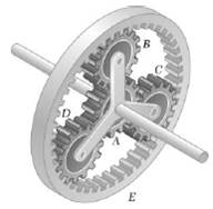 Example 2: An ‘epicyclic’
gearbox is a special arrangement of gears that has many applications. The sketch shows a simple example. The gearbox can be driven in three different
places: one drive shaft is connected to the central sun gear (A); the other is
attached to the ‘planet carrier’, which is joined to the center of the ‘pinion
gears’ B,C and D. The outer gear (E called the ‘ring gear’) can also be driven
separately.
Example 2: An ‘epicyclic’
gearbox is a special arrangement of gears that has many applications. The sketch shows a simple example. The gearbox can be driven in three different
places: one drive shaft is connected to the central sun gear (A); the other is
attached to the ‘planet carrier’, which is joined to the center of the ‘pinion
gears’ B,C and D. The outer gear (E called the ‘ring gear’) can also be driven
separately.
Epicyclic gearboxes are used in all automatic vehicle
transmissions. They are also very
useful in ‘split power’ drives, where two motors need to be connected together
to drive a single axle. Hybrid
vehicles, which have both an electric motor and an internal combustion engine
driving the same axle, are one example.
You can find a very nice description of the Toyota Prius split power
transmission here: the website
includes a Flash animation that lets you change the speeds of the motors in the
system and visualize the motion of the gears.
 The figure shows a schematic diagram illustrating the
general geometry and motion of the system.
We have four rigid bodies:
The figure shows a schematic diagram illustrating the
general geometry and motion of the system.
We have four rigid bodies:
- The central sun gear, radius , teeth, rotating at angular velocity
- The planet carrier, angular
velocity
- The ring gear, radius ,
with teeth, angular velocity
- The planet gear, radius , teeth, rotating at angular velocity
In any application, we are given the angular velocity of two of the
drive shafts (any two of ,
,
), and must calculate the third. The planet gear is not connected to any drive
shaft, so we usually don’t care very much about its angular speed, but we will
need to find to solve for the unknown one of ,
,
.
This seems a terribly difficult problem, but it can be solved in a very
simple way with a trick.
 We start by solving a simpler version of the
problem. Suppose that the planet carrier
is stationary ( =0) and the sun gear rotates with angular
speed (see the animation). What is the angular
velocity of the ring gear?
We start by solving a simpler version of the
problem. Suppose that the planet carrier
is stationary ( =0) and the sun gear rotates with angular
speed (see the animation). What is the angular
velocity of the ring gear?
The sun gear and the planet gear are just a standard gear pair so we
know that
The two touching points on the planet gear and the ring gear must have
the same velocity, so (using the rotating gear formula)
We can eliminate to get the answer:
Now let’s try the harder problem.
The animation shows a general situation, where ,
are both nonzero. How can we find now?
 This is difficult to analyze because the center of the
planet gear is not fixed, so it’s hard for us to visualize the motion, and the
standard gear formulas don’t work. But
we can simplify the problem by analyzing motion in a reference frame that
rotates with the planet carrier. For
example, imagine attaching a videocamera to the planet carrier this camera would show the planet carrier to
be stationary, with the surrounding world rotating in the opposite
direction. The angular velocity of the planet carrier would be subtracted from all
the other angular velocities. In
this reference frame, we can use the result we just calculated:
This is difficult to analyze because the center of the
planet gear is not fixed, so it’s hard for us to visualize the motion, and the
standard gear formulas don’t work. But
we can simplify the problem by analyzing motion in a reference frame that
rotates with the planet carrier. For
example, imagine attaching a videocamera to the planet carrier this camera would show the planet carrier to
be stationary, with the surrounding world rotating in the opposite
direction. The angular velocity of the planet carrier would be subtracted from all
the other angular velocities. In
this reference frame, we can use the result we just calculated:
This result is general, and can be re-arranged to tell
you the angular velocities for any given combination of ,
and .
6.4 Linear
momentum, angular momentum and kinetic energy of rigid bodies
 In this section, we determine how to calculate the
angular momentum and kinetic energy of a rigid body, and define two important
quantities: (1) the center of mass of a rigid body (which you already know),
and (2) the Inertia tensor (matrix) of a rigid body.
In this section, we determine how to calculate the
angular momentum and kinetic energy of a rigid body, and define two important
quantities: (1) the center of mass of a rigid body (which you already know),
and (2) the Inertia tensor (matrix) of a rigid body.
To keep things simple, we won’t consider a general
rigid body right away. Instead, we will
calculate the linear momentum, angular momentum, and kinetic energy of a system
of N particles that are connected
together by rigid, massless links.
Definitions
of inertial properties: For this system, we will define
The total mass
The position of
the center of mass
The position
vector of each mass relative to the center of mass
The velocity of
the center of mass
The mass moment
of inertia about the center of mass (a tensor, which can be expressed as a
matrix if we choose a coordinate system and set )
The mass moment of inertia is sometimes also written in a more abstract
but very compact way as
Here, is the identity tensor, and is a tensor with components , ,
,
etc (the symbol is called the ‘diadic product’ of two vectors).
Formulas for linear and angular momentum
and kinetic energy: We will show that:
The total linear momentum is
The total angular momentum (about the origin) is
The total kinetic energy is
These are actually general results that hold for all rigid bodies, as
long as we use a more general definition of and .
 Simplified
formulas for two dimensions: For planar
problems, (since all the masses are in the plane), and . In
this case, we can use
Simplified
formulas for two dimensions: For planar
problems, (since all the masses are in the plane), and . In
this case, we can use
The total linear momentum is
The total angular momentum (about the origin) is
The total kinetic energy is
Here is just the bottom diagonal term of the full
inertia matrix (i.e. just a single number)
 Example 1: A simple 3D
assembly of masses is shown in the figure.
Example 1: A simple 3D
assembly of masses is shown in the figure.
(1) Find the mass moment of inertia.
By symmetry, the COM is at the origin. The inertia tensor is therefore
(2) Assume that the COM is stationary (i.e. the
assembly rotates about the origin). Find formulas for the angular momentum and
kinetic energy of the system, in terms of the angular velocity components
The formula gives the angular momentum
Note that h is a
vector. Importantly, h is not generally parallel to the
angular velocity vector, as this example shows.
The kinetic energy is
These results help us understand what the formulas are predicting. Note, for example, that:
·
The mass moment
of inertia always has the form mass*length2. It has units of kg-m2
·
The mass moment
of inertia is a measure of how mass is distributed about the center of
mass. An object has a large inertia if
the mass is far from the COM, and a small one if the mass is close to the COM.
·
 The matrix-vector products in the formulas for h and T are really just a way of calculating the velocity of each
particle in the system in a quick way. For
example, suppose we rotate our assembly of masses about the k axis with angular velocity (see the animation). Let’s calculate the kinetic energy of the
system, but without using the rigid body formulas. The two blue masses are stationary, so they
have no KE. The red and green mass are
both moving in a circle about the origin.
The circular motion formula says their speed is We can calculate the total kinetic energy
using the usual formula
The matrix-vector products in the formulas for h and T are really just a way of calculating the velocity of each
particle in the system in a quick way. For
example, suppose we rotate our assembly of masses about the k axis with angular velocity (see the animation). Let’s calculate the kinetic energy of the
system, but without using the rigid body formulas. The two blue masses are stationary, so they
have no KE. The red and green mass are
both moving in a circle about the origin.
The circular motion formula says their speed is We can calculate the total kinetic energy
using the usual formula
This explains why the formula for contains and - the component keeps track of how much energy or
momentum is produced by a rotation about the z axis. The energy and
momentum depend on the distances of the masses from the z axis which of course depends on and .
Finally, note that we can interpret the two terms in
the formulas for momentum and KE as quantifying (separately) the effects of
translation and rotation
Angular momentum
Kinetic energy is
This helps explain why we can often idealize a system
as a particle. If the rotational term is
negligible, the angular momentum and kinetic energy of a rigid body is just the
same as that of a particle located at the COM.
6.4.1 Deriving the linear momentum
formula
By definition . We can re-write this as follows:
(we used the definition of the COM to get the last result)
6.4.2 Deriving the angular momentum
formula
Start with the definition:
Note that and recall the relative velocity formula . This
means we can re-write the angular momentum as
Note that
Finally, recall the dreaded triple cross product formula
This means that
This gives us the result in compact notation directly
where we used the compact formula for the mass moment of inertia about
the COM:
If you don’t like the compact formula, we can also get the matrix
version by expand out the triple cross product
This again shows that
Finally collecting terms gives the required answer
6.4.3 Deriving the kinetic energy
formula
We can use
Recall that
and expand the dot product of two cross products using the formula
This shows that
As for the derivation of the angular momentum, this can be rearranged
using the compact notation as
Alternatively, we can get the matrix version of the formula as
Finally, collecting all the terms gives the required answer
6.4.4 Calculating the center of mass and
inertia of a general rigid body
It is not hard to extend the results for a system of N particles to a general rigid
body. We simply regard the body to be
made up of an infinite number of vanishingly small particles, and take the
limit of the sums as the particle volume goes to zero. The sums all turn into integrals.
3D problems: For a body with mass density (mass per unit volume) we have that
 The total mass is
The position of the center of mass is
The mass moment of inertia about the center of
mass is
where
 For 2D
problems: We know the COM must lie in the i,j plane and we don’t need to calculate the whole matrix.
For 2D
problems: We know the COM must lie in the i,j plane and we don’t need to calculate the whole matrix.
For a body with mass per unit area we can therefore use the formulas
 The total mass is
The position of the center of mass is
The mass moment of inertia about the center of
mass is
where
 Example 1: To show how to
use these, let’s calculate the total mass, center of mass, and mass moment of
inertia of a rectangular prism with faces perpendicular to the axes:
Example 1: To show how to
use these, let’s calculate the total mass, center of mass, and mass moment of
inertia of a rectangular prism with faces perpendicular to the axes:
First the total mass (sort of trivial)
Now the COM
And finally the mass moment of inertia
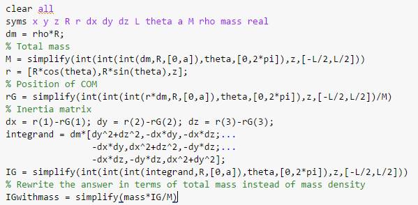
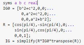
 Example 2: As a second
example, let’s calculate the mass moment of inertia of a cylinder with mass
density , length L
and radius a. We have to do the integrals with polar
coordinates. For example, the inertia matrix is
Example 2: As a second
example, let’s calculate the mass moment of inertia of a cylinder with mass
density , length L
and radius a. We have to do the integrals with polar
coordinates. For example, the inertia matrix is
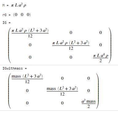
Now (in polar coordinates, and assuming that the COM is located at the
center of the cylinder) .
We can have Matlab do all the integrals for us:
 Example 3: Let’s finish up
with a 2D example. Find the mass,
center of mass, and out of plane mass moment of inertia of the triangle shown
in the figure.
Example 3: Let’s finish up
with a 2D example. Find the mass,
center of mass, and out of plane mass moment of inertia of the triangle shown
in the figure.
The total mass is
The position of the COM is
The 2D mass moment of inertia is
This is all a big pain, and you may be contemplating a
life of crime instead of an engineering career. Fortunately, it is very rare to have to do
these sorts of integrals in practice, because all the integrals for common
shapes have already been done. You can
google most of them. The tables below
give a short list of all the objects we will encounter in this course.
Table of mass moment of inertia tensors for selected
3D objects
|
Prism
|
|
|
|
Solid Cylinder
|
|
|
|
Solid Cone
|
|
|
|
Solid Sphere
|
|
|
|
Solid Ellipsoid
|
|
|
|
Hollow Cylinder
|
|
|
Table of mass moment of inertia about perpendicular
axis for selected 2D objects
|
Square
|
|
|
|
Disk
|
|
|
|
Thin ring
|
|
|
|
Hollow disk
|
|
|
|
Slender rod
|
|
|
6.4.5 The Parallel Axis Theorem
In all the previous calculations we have been
calculating the mass moment of inertia about the center of mass. This is what always appears in the general angular
momentum formula. But we sometimes want
to find the mass moment of inertia about a different
point (not the COM). For example, if a
body happens to be rotating about a fixed point, we can sometimes find its
angular momentum and kinetic energy more quickly by first finding the mass
moment of inertia about the fixed point, and then using special simpler
formulas the angular momentum and kinetic energy (see section 6.4.10). We also sometimes want to find the combned
mass moment of inertia of several bodies that are connected together. When we do this, we usually find the center
of mass of the collection of bodies, and then add up the mass moments of
inertia of all the separate bodies about the COM of the assembly (see section
6.4.6). To be able to do this, we need
to be able to calculate the mass moment of inertia of a body about and
arbitrary point, i.e. not the COM of the body.
 The mass moment of inertia about an arbitrary point is
defined exactly the same way as the inertia about the COM, except that we use
the distances from our arbitrary point instead of the distance from the COM.
The mass moment of inertia about an arbitrary point is
defined exactly the same way as the inertia about the COM, except that we use
the distances from our arbitrary point instead of the distance from the COM.
It’s painful to have to re-do all these integrals, however. If we already know , the parallel axis theorem lets us calculate directly.
Define the vector d that
points from G to O
Then for a 3D object with mass M
For 2D we have a simpler result
 Example: Let’s find the
mass moment of inertia of a cylinder about axes that pass through one end of
the cylinder (O), instead of the COM.
Example: Let’s find the
mass moment of inertia of a cylinder about axes that pass through one end of
the cylinder (O), instead of the COM.
Here,
The formula gives
Proof of the parallel axis theorem
 Let be some arbitrary point in space, and let be the position of the COM. Define as the vector from the COM to O, as shown in
the figure.
Let be some arbitrary point in space, and let be the position of the COM. Define as the vector from the COM to O, as shown in
the figure.
Then let denote the position vector of an infinitesimal
volume element in the rigid body relative to O, and let denote the position vector of the same volume
element relative to the COM G. Then .
We also know that (by definition)
We can make use of and then substitute into (1).
Expand the dot and dyadic product of ,
note d is a constant and use the
identities on the last line above, as follows
6.4.6 Calculating moments of inertia of
complex shapes by summation
The most important application of the parallel axis
theorem is in calculating the mass moment of inertia of complicated objects
(which don’t appear in our table) by adding together moments of inertia for
simple shapes. We can illustrate this
with a couple of simple examples.
Example 1: Two spheres with radius 3a are connected by a rigid cylinder with length 6a and radius a to create a dumbbell. All
objects have the same mass density .
Calculate the total mass moment of inertia of the dumbbell.
The general approach is
(1)
Find the COM of
the entire assembly
(2)
Find the mass
moment of inertia of each shape (the spheres and the cylinder) about its own
COM
(3)
Use the parallel
axis theorem to find the moment of inertia of each shape about the combined COM
(4)
Add all the
moments of inertia
For our problem
(1)
We know the COM
is at the origin by symmetry, so we don’t need to calculate it
(2)
The inertia
matrices of each object (cylinder + sphere) about their own COM are:
(3)
We don’t need to
use the parallel axis theorem for the cylinder, because its COM is already at
the same place as the COM of the assembly.
For the spheres, we need to move the COM a distance 6a parallel to the k direction. This means that in our formula. Therefore
(4)
We can add
everything up (note that there are two spheres). Its best to use Mupad. The answer is
Example 2: Things are a lot simpler in 2D. The procedure is the same, but we only need
to calculate . For
example, to calculate the mass moment of inertia for a square 2ax2a plate with a hole with an axa square cut out from the top corner we would use the following approach.
Start by calculating the total mass and the position of the COM. We can regard the cut-out section as a square
with negative density inside a larger 2ax2a square.
The total mass is therefore
The position of the COM is
The mass moment of inertia of the 2ax2a square and the axa square are
We now use the parallel axis theorem to find the moment of inertia of
each square about the combined COM. For
the large square: . For
the small square, . The total mass moment of inertia is therefore
6.4.7 Rotating the inertia tensor
All
the curious properties of spinning objects a gyroscope; a boomerang; the rattleback are consequences of the fact that the mass moment
of inertia of an object changes when it is rotated. We can see this very easily by
re-visiting our assembly of masses. In
the original calculation, the red, green and blue masses were located on the i,j,k axes. We calculated the inertia
tensor to be
Now
suppose we rotate the assembly through 90 degrees about the k axis.
The red masses now lie on the j axis,
and the green ones line up with the i
axis. It is not hard to see that the
new mass moment of inertia is now
( have switched positions)
This
seems like a huge problem if we needed to re-calculate the mass moment
of inertia from scratch every time a rigid body moves, analyzing rigid body
motion would be nearly impossible.
Fortunately,
we can derive a formula that tells us how the mass moment of inertia of a body
changes when it is rotated.
 Rotation
formula for moments of inertia: Consider
the rectangular prism shown in the figure.
Let denote the mass moment of inertia with the
prism oriented so the faces are perpendicular to i,j,k (i.e. the inertia given in the table in Sect 6.4.5).
Rotation
formula for moments of inertia: Consider
the rectangular prism shown in the figure.
Let denote the mass moment of inertia with the
prism oriented so the faces are perpendicular to i,j,k (i.e. the inertia given in the table in Sect 6.4.5).
Suppose
the body is then rotated by a tensor R.
The mass moment of inertia
after rotation is given by
Example: The prism shown in the figure is rotated by 45 degrees
about the k axis. Calculate the mass moment of inertia after
the rotation
Start by calculating the
rotation (use the formulas from 6.2.1)
We know the inertia tensor of
the prism before it is rotated is
We can use Matlab to do the
tedious matrix multiplications
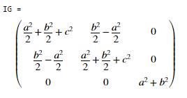
Note that the inertia tensor
is no longer diagonal.
 Rotation
formula for 2D motion: Fortunately, 2D
is simple
Rotation
formula for 2D motion: Fortunately, 2D
is simple
Rotating a 2D object about the k axis does not change
Proof of the rotation formula: Consider a system of N particles. Suppose that
before rotation, the particles are at positions relative to the COM. The initial inertia tensor is
Now rotate the system, so the
particle s move to new positions . The new inertia tensor is
Recall that and recall that a rotation R does not change lengths so . Therefore
It is easy to show (just
write out the matrix products) ,
which shows that
6.4.8 Time derivative of the inertia tensor
When
we analyze motion of a rigid body, we will need to calculate the time
derivatives of the linear and angular momentum. Linear momentum is no problem, but for angular
momentum, we will need to know how to differentiate with respect to time. There is a formula for this:
where is the
spin tensor (see sect 6.2.2)
Proof:
- Start with and take the time derivative
- Recall that
- Finally note that and therefore
6.4.9 Time derivative of angular momentum
To
use the angular momentum conservation equation, we will need to know how to
calculate the time derivative of the angular momentum. When we do this for a 3D problem, we need to
take into account that the mass moment of inertia changes as the body rotates. We will prove the following formula:
For 2D planar problems this can be simplified to:
Proof: We
start by taking the time derivative of the general definition of h
We can go ahead and do the
derivative with the product rule:
We can simplify this by
noting that and of course the cross product of with itself is zero. We can also use the definition of angular
acceleration: . This
gives
Finally, substitute for from the formula in the previous section, and
recall that for all vectors u, and that a vector crossed with itself is zero to see that:
6.4.10 Special equations for angular momentum and KE
of bodies that rotate about a stationary point
We
often want to predict the motion of a system that rotates about a fixed pivot a pendulum is a simple example. These problems can be be solved using a
useful short-cut for the angular momentum or KE of a body rotating about a
fixed point. The short-cut will give
the same answer as the general formulas.
For an object that rotates about a fixed pivot at the
origin:
The total angular momentum (about the origin)
is
The total kinetic energy is
Here
is the mass moment of inertia about O
(calculated, eg, using the parallel axis theorem). Note that the special formulas do not include the term involving the
velocity of the COM that’s been automatically included by using instead of .
For 2D rotation about a fixed point at the origin we can simplify these to
 The total angular momentum (about the origin)
is
The total angular momentum (about the origin)
is
The total kinetic energy is
Proof: It
is straightforward to show these formulas.
Let’s show the two dimensional version of the kinetic energy formulas as
an example. For fixed axis rotation, we can use the rigid body formulas to
calculate the velocity of the center of mass (O is stationary and at the
origin)
The general formula for
kinetic energy can therefore be re-written as
The
other formulas can be proved with the same method we simply express the velocity or acceleration
of the COM in the general formulas in terms of angular velocity and
acceleration, and notice that we can re-arrange the result in terms of the mass
moment of inertia about O.
The 3D proof is the
same. Start with the general formula
and use the kinematics
formula to find (noting
that O is stationary and at the origin)
Remember the vector formula ,
which shows that
We can re-write the kinetic
energy as
using the parallel axis
theorem.
Another way to prove the
result is just to calculate the KE of the body from scratch, by summing the KE
of the infinitesimal particles in the rigid body, and noting that they are all
in circular motion about O.
The proof of the angular
momentum formula is just the same start with the general formula for h and then simplify it using . You might like to try this as an exercise.
Example: In
the planetary gear system shown, the sun gear has radius and mass m
, the ring gear has radius , while the planet gear has mass m and the planet carrier has mass m/2 .
The sun gear rotates with angular speed and the ring gear is stationary.
Find a formula for the total angular momentum of the assembly about the
center of the sun gear, in terms of ,
and m. Treat the gears as disks, the planet carrier
as a 1D rod and assume there’s only one planet gear as shown to keep things
simple; this would be a rather unusual gear system but adding more gears just
makes the problem tedious without illustrating any new concepts...
The 2D formula for
angular momentum of a rigid body (about the origin) is
where is the position vector of the COM of the body
relative to the origin.
We need to find the angular speed of all the moving
parts: using the gear formulas
we
see that
and
The
COM of the planet carrier is half way along its length; its COM is in circular
motion with speed
Similarly
the COM of the planet gear is in circular motion with speed
Now
we can add up all the angular momenta:
1. Sun
2. Planet carrier
Notice
that the planet carrier rotates about the
center of the sun. So, if we want, we
could also use the special formula for
angular momentum of an object rotating about a fixed point
where
is the mass moment of inertia of the planet
carrier about the fixed point, which must be calculated using the parallel axis
theorem
(where
we noted that the length of the bar is ). We
know so
as
before.
3. Planet gear
Note that we can’t
use the special formula for rotation about a fixed point for the planet gear,
because although there is a fixed point on the planet gear (where it touches
the ring), we were asked to find the angular momentum about the center of the
sun. This is not a fixed point on the planet gear.
Sum
everything