Chapter 6
Rigid Body Dynamics
6.5 Rotational forces review of moments exerted by forces and torques
You
can find a detailed discussion of forces and moments, with lots of examples, in
Section 2 of these notes. Moments and
torques don’t come up very often in particle dynamics, but play a very
important role in rigid body dynamics. We
therefore review the most important concepts related to torques and moments
here.
You need to remember, and
understand, these ideas:
(1) A moment is a generalized force that
causes an object to rotate (see section 2).
(2) A force can exert a moment on a rigid body. The moment
of a force (about the origin) is defined as
(3)
In general, a
force causes a rigid body to accelerate, and will also induce an angular
acceleration (so it influences both translational and rotational motion).
(4)
A ‘torque’ or
‘pure moment’ is a special kind of generalized force that causes an object to
rotate, but has no effect on its translational motion. As an
example, a motor shaft (eg the bit on a power-driven screwdriver!) will exert a
torque on the object connected to it.
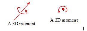
(5)
A torque or pure
moment is a vector quantity it has magnitude and direction. The direction indicates the axis associated
with its rotational force (following the right hand screw convention); the
magnitude represents the intensity of the rotational force. The magnitude of a
torque has units of Newton Meters. A moment is often denoted by the symbols
shown in the figure
6.5.1 Rate of work done by a torque or
moment: If a torque acts
on an object that rotates with angular velocity ,
the rate of work done on the object by Q
is
6.5.2 Torsional springs

A
solid rod is a good example of a torsional spring. You could take hold of the
ends of the rod and twist them, causing one end to rotate relative to the
other. To do this, you would apply a moment or a couple to each end of the rod, with direction parallel to the axis
of the rod. The angle of twist
increases with the moment. Various
torsion spring designs used in practice are shown in the picture the image is from
http://www.mollificio.lombardo.molle.com/springs/torsion_springs.html
More
generally, a torsional spring resists rotation, by exerting equal and opposite
moments on objects connected to its ends.
For a linear spring the moment is proportional to the angle of rotation
applied to the spring.
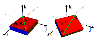
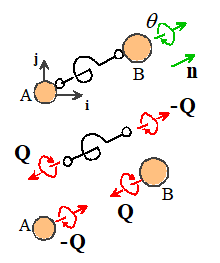 The figure shows a formal free body diagram for two
objects connected by a torsional spring.
If object A is held fixed, and
object B is rotated through an angle about an axis parallel to a unit vector n, then the spring exerts a moment
The figure shows a formal free body diagram for two
objects connected by a torsional spring.
If object A is held fixed, and
object B is rotated through an angle about an axis parallel to a unit vector n, then the spring exerts a moment
on object B where is the torsional
stiffness of the spring. Torsional
stiffness has units of Nm/radian.
The
potential energy of the moments exerted by the spring can be determined by
computing the work done to twist the spring through an angle .
- The work done by a
moment Q due to twisting
through a very small angle about an axis parallel to a vector n is
- The potential energy is the negative of the total
work done by M, i.e.
A
potential energy cannot usually be defined for most concentrated moments,
because rotational motion is itself path dependent (the orientation of an
object that is given two successive rotations depends on the order in which the
rotations are applied).
6.6 Dynamics of rigid bodies
 We predict the position and velocity of a particle by
integrating F=ma. For a rigid body, we
need to predict both its position and orientation. We use the following equations to do this.
We predict the position and velocity of a particle by
integrating F=ma. For a rigid body, we
need to predict both its position and orientation. We use the following equations to do this.
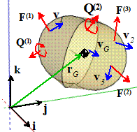
The figure shows a rigid body
subjected to several forces and torques (pure moments) .
During a representative time interval the forces exert a linear impulse and angular impulse A, and do total work on the rigid body .
The body has total mass M and mass moment of inertia about the center of mass.
Let denote the position, velocity and acceleration
of the center of mass, and let denote the angular velocity and
acceleration.
The linear and angular
momentum (about the origin) of the rigid body follow as , , and its kinetic energy is .
The equations of motion are
then
Force-acceleration relation:
Moment angular velocity/acceleration relation
Force-momentum and impulse-momentum relation:
Moment angular momentum relation:
Power work kinetic energy relation
For 2D planar motion we can use the simplified formulas
Derivations: It is possible
to obtain the equations of motion for a rigid body from Newton’s laws for a
particle the basic idea is to assume that a rigid body
consists of an infinite number of particles connected by rigid massless links but this isn’t really a rigorous proof,
because we have to assume that the links are two-force members, and there is no
way to prove that this is a realistic description of matter. Another viewpoint is to accept conservation
of linear momentum and angular momentum as two separate physical laws (the
linear momentum is just Newton’s law, and the angular momentum equation is
sometimes referred to as Euler’s law). We can then ‘prove’ that a rigid body
can be represented as a bunch of particles connected by two force members. We’ll show the first approach here.
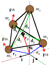
The figure shows a system of
particles connected by rigid massless links.
The length of the link between the ith and jth particle will be denoted
by We assume that all the links are two-force
members.
The particles are subjected
to a set of external forces . We
denote the magnitude of the force in the member connecting the ith and jth particle by (by convention a positive represents an attractive force between the
particles). Note that the because the two particles exert equal and opposite forces on
each other. The vector valued force
exerted on the ith particle by the jth
follows as
(to see this note that is a unit vector from the ith to the jth
particles)
We can start the derivation
with the force-linear momentum relation for a single particle. For example, for the ith particle (see section 4 of the notes)
Sum this over all particles
But we know that ,
and since the second term on the left hand side is
zero. Therefore
Since this is independent of
the number of particles, it must also apply to a rigid body. This shows that the force-momentum and
force-acceleration for a rigid body can be derived from Newton’s law for a
particle.
We can derive the angular
momentum relation for a rigid body using the same idea. For one particle we have the angular momentum
equation
where we have noted that . We
can sum this over all the particles
The second term here is zero,
because and (just write out the sum term by term for some
finite number of particles eg two if you don’t see this). The term on the right hand side is clearly
just the total angular momentum of the system.
If we replace some subset of the forces with a statically equivalent
torque and force, we obtain the moment-angular momentum equation.
6.7 Summary of equations of motion
for rigid bodies
In
this section, we collect together all the important formulas from the preceding
sections, and summarize the equations that we use to analyze motion of a rigid
body.
We
consider motion of a rigid body that has mass density during some time interval , and define the following quantities:
6.7.1
Forces,
torques, impulse, work, power
 The total force acting on the body
The total linear impulse exerted by forces during
the time interval
The total moment (including torques) acting on
the body
The tot al angular impulse exerted on the body
during the time interval
The rate of work done by forces and torques
acting on the body
The total work done by forces and torques on
the body during the time interval
6.7.2 Inertial properties
The total mass is
 The position of the center of mass is
The mass moment of inertia about the center of
mass
where
 For a 2D body with mass per unit area we use
 The total mass is
The position of the center of mass is
The mass moment of inertia about the center of
mass is
where
6.7.3 Describing motion
The rotation tensor (matrix) maps the vector
connecting two points in a solid before it moves to its position after motion
The spin tensor is related to R by
Rotation through an angle about an axis parallel to a unit vector
is
The angular velocity vector is related to W by
The angular acceleration vector is
The velocities of two points A and B in a
rotating rigid body are related by
The accelerations of A and B are related by
6.7.4 Momentum and Energy
The total linear momentum is
The angular momentum (about the origin) is
The total kinetic energy is
For
2D planar problems, we know . In
this case, we can use
The total linear momentum is
The total angular momentum (about the origin)
is
The total kinetic energy is
6.7.5 Conservation laws
Linear momentum
Angular momentum
Work-Power - Kinetic Energy relation
Energy equation for a conservative system
6.7.6 Linear and angular momentum equations in terms
of accelerations
The linear and angular
momentum conservation equations can also be expressed in terms of
accelerations, angular accelerations, and angular velocities. The results are
For 2D planar motion we can use the simplified formulas
6.7.7 Special equations for analyzing bodies that
rotate about a stationary point
We
often want to predict the motion of a system that rotates about a fixed pivot a pendulum is a simple example. These problems can be solved using the
equations in 6.6.5 and 6.6.6, but can also be solved using a useful short-cut.
For an object that rotates about a fixed pivot at the
origin:
The total angular momentum (about the origin)
is
The total kinetic energy is
The equation of rotational motion is
Here is the mass moment of inertia about O
(calculated, eg, using the parallel axis theorem)
For 2D rotation about a fixed point at the origin we can simplify these to
 The total angular momentum (about the origin)
is
The total angular momentum (about the origin)
is
The total kinetic energy is
The equation of rotational motion is
Proof: It
is straightforward to show these formulas.
Let’s show the two dimensional version of the kinetic energy formulas as
an example. For fixed axis rotation, we can use the rigid body formulas to calculate
the velocity of the center of mass (O is stationary and at the origin)
The general formula for
kinetic energy can therefore be re-written as
The
other formulas can be proved with the same method we simply express the velocity or acceleration
of the COM in the general formulas in terms of angular velocity and
acceleration, and notice that we can re-arrange the result in terms of the mass
moment of inertia about O.
6.8 Examples of solutions to problems involving motion
of rigid bodies
The best way to learn how to
use the equations in section 6.6 is just to work through a series of examples.
6.8.1 Solutions to 2D problems
 Example 1: A solid of
revolution (eg a cylinder or sphere) with mass M and mass moment of inertia about its COM is
released from rest at the top of a ramp.
It rolls without slip. Calculate
its velocity at the bottom of the ramp.
Example 1: A solid of
revolution (eg a cylinder or sphere) with mass M and mass moment of inertia about its COM is
released from rest at the top of a ramp.
It rolls without slip. Calculate
its velocity at the bottom of the ramp.
- The system is conservative, so we can solve the problem using
energy conservation. The energy
equation tells us that the sum of kinetic and potential energy of the
cylinder is constant:
- We can take the datum for potential energy to be the position of
the COM at the bottom of the ramp. The initial potential energy is
therefore ; the final potential energy is zero.
- The initial kinetic energy is zero, because the cylinder is
stationary. The final kinetic
energy is .
- The energy equation gives
- Finally, since the cylinder rolls without slip, we know that .
Hence
This formula predicts that an
object with a smaller inertia will move faster than an object with a large
inertia. A sphere rolls down the ramp
more quickly than a cylinder, for example, and a solid cylinder rolls more
quickly than a ring.
 Example 2: For the
problem treated in the preceding section, calculate the critical value of
friction coefficient necessary to prevent slip at the contact.
Example 2: For the
problem treated in the preceding section, calculate the critical value of
friction coefficient necessary to prevent slip at the contact.
If we want to learn about
forces, we have to use the linear and angular momentum equations. This problem can be solved with the 2D
formulas in terms of accelerations:
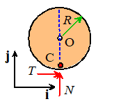
- The figure shows a free body diagram for the cylinder (or sphere)
- We know that the COM is always a constant height above the ramp,
so the acceleration must be parallel to i. The linear momentum
equation gives
- We can use the angular momentum equation it is convenient to take moments about
the contact point C. (There are no
torques in this problem).
- Finally, we can use the rolling wheel formula for accelerations .
- The preceding results give:
- Finally, substituting back into the i components of (1):
- The j component of (1)
gives
- For no slip
The
formula shows that objects with large values of are more likely to slip. If the inertia is very small, slip will
never occur. A ring will slip on a
lower slope than a cylinder, which will slip on a lower slope than a sphere.
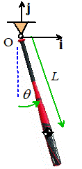
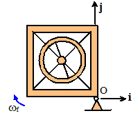
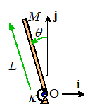 Example 3: A vertical
mast can be idealized as a slender rod with length L and mass M, which is
held in an inverted position by a torsional spring with stiffness at its base.
Find the equation of motion for the angle in the figure, and hence determine the natural
frequency of vibration of the mast.
Example 3: A vertical
mast can be idealized as a slender rod with length L and mass M, which is
held in an inverted position by a torsional spring with stiffness at its base.
Find the equation of motion for the angle in the figure, and hence determine the natural
frequency of vibration of the mast.
This is a conservative system. Also, the mast rotates about a fixed
point. We can analyze the problem using
energy methods, and use the special formulas for rotation about a fixed point.
·
The kinetic
energy formula for planar motion is
·
For planar motion
we know that
·
We can use the
parallel axis theorem to calculate the mass moment of inertia of a rod about
one end:
·
Gravity and the
torsional spring both contribute to the total potential energy of the system. The total potential energy is
·
Energy
conservation means that
·
Recall that so
·
We assume that is small enough that , so
·
This is a
standard ‘Case I’ undamped vibration EOM, so we can just read off the natural
frequency
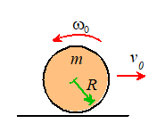
Example 4: A thin uniform disk of radius R, mass m and mass moment
of inertia is placed on the ground with a positive
velocity in the horizontal direction, and a
counterclockwise rotational velocity (a backspin) . The contact between the disk and the ground
has friction coefficient .
The disk initially slips on the ground, and for a suitable range of values of and its direction of motion may reverse. The goal of this problem is to calculate the
conditions where this reversal will occur.
 General
discussion of slipping contacts: Solving problems with sliding at a contact is always
tricky, because we have to draw the friction forces in the correct
direction. Before tackling the example,
we will summarize the general rules. We
will consider a wheel as an example, but the rules apply to contact between any
object and a stationary surface. The
figure shows a wheel that spins with angular velocity while the center moves with speed . The
direction of the friction force is determined by the direction of motion of the
point on the wheel that instantaneously touches the ground, which can be
calculated from the formula
General
discussion of slipping contacts: Solving problems with sliding at a contact is always
tricky, because we have to draw the friction forces in the correct
direction. Before tackling the example,
we will summarize the general rules. We
will consider a wheel as an example, but the rules apply to contact between any
object and a stationary surface. The
figure shows a wheel that spins with angular velocity while the center moves with speed . The
direction of the friction force is determined by the direction of motion of the
point on the wheel that instantaneously touches the ground, which can be
calculated from the formula
Friction
always acts to try to bring point C to rest if C is moving to the right, friction acts to
the left; if C is moving to the left, friction acts to the right.
There
are three possible cases:
Forward slip: Point
C moves in the positive i direction
over the ground

Slip occurs at the contact,
We have to use the friction law
Point C is moving to the right, so friction
must act to the left
Pure rolling . Point
C is stationary.

No slip occurs at the contact.
In this case
We can draw the friction force in either
direction at the contact (if we choose the wrong direction, our calculations
will just tell us that T is
negative). It is usually convenient to
choose T to act in the positive i direction, but this is not necessary.
Reverse slip: Point
C moves in the negative i direction
over the ground
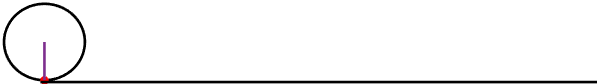
Slip occurs at the contact,
We have to use the friction law
Point C is moving to the left, so friction
must act to the right
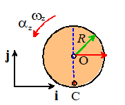
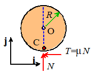
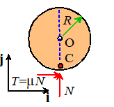
Now we return to the example.
4.1 Draw a free body diagram showing the forces acting
on the disk just after it hits the ground.
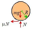 We are given that and are both positive so we have . This is forward slip, and we use the
corresponding FBD.
We are given that and are both positive so we have . This is forward slip, and we use the
corresponding FBD.
4.2 Hence, find formulas for the initial acceleration and angular acceleration for the disk, in terms of g , R and . Note that the contact point is slipping.
The equations of
motion are
Solving these and using :
4.3 Find formulas for the velocity and angular velocity of
the disk, during the period while the contact point is still slipping.
The acceleration and
angular acceleration are constant, so we can use the constant acceleration
formulas:
4.4 Find a formula for the time at which the disk will
reverse its direction of motion.
Velocity is reversed
where v=0. From the previous part, at the reversal.
4.5 Find a formula for the time at which the disk begins
to roll on the ground without slip.
Hence, show that the disk will reverse its direction only if
Rolling without
sliding starts when . We have that
The reversal will only
occur if rolling without slip occurs after the reversal of velocity. This means
Example 5: The
‘Sweet Spot’ on a softball or baseball bat, or tennis or squash racket is a
point that minimizes the reaction forces acting on the athlete’s hand when the
ball is struck. In fact, any rigid body
has a sweet spot the magic point is called the ‘center of
percussion’ of a rigid body.
For baseball and
softball bats in particular, there is a standard ASTM test that can
be used to measure the position of the sweet spot. The test works like this: the bat is
suspended from the knob on handle, so it swings like a pendulum. The period of vibration of the swinging bat is then measured. ASTM say that the center of percussion is
then a distance
 from the end of the handle. Why does this work? It seems that this test has nothing whatever
to do with a ball hitting the bat!
from the end of the handle. Why does this work? It seems that this test has nothing whatever
to do with a ball hitting the bat!
We will solve this problem in two parts. First, we will calculate a formula for the period
of vibration in the ASTM test. Then we
will calculate the position of the center of percussion. We will see that the ASTM test does indeed
make the correct prediction.
We can calculate the period
using the energy method. The figure
shows the ASTM pendulum test. We assume
that
·
The bat has a
mass moment of inertia about its COM
·
The COM is a
distance L from O
The bat pivots about O, so
we can use the fixed axis rotation formula for the kinetic energy
Here (using the parallel axis theorem).
The potential energy
is .
Energy conservation gives
If is small then so the equation of motion reduces to
This is a standard ‘Case 1’
EOM. The natural frequency is so the period is
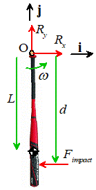 Next, we find the position of the ‘sweet spot’. We can
do this by calculating the reaction forces on the handle when the bat is
struck, and finding the impact point that minimizes the reaction force.
Next, we find the position of the ‘sweet spot’. We can
do this by calculating the reaction forces on the handle when the bat is
struck, and finding the impact point that minimizes the reaction force.
The
figure shows an impact event. We assume
that:
- The bat rotates in the horizontal plane (so
gravity acts out of the plane of the figure).
- The bat rotates about the point O
- The ball impacts the bat a distance d from the handle.
- The ball exerts a (large) force on the bat
- Reaction forces act on the handle during the impact.
This
is a planar problem, so we can use the 2D equations of motion. The equation for
translational motion gives
For
the rotational equation we can also use the short-cut for fixed axis rotation
We can relate to using the rigid body formula:
We therefore see that
The sweet spot is at
the position that makes , which shows that
For comparison, the
ASTM formula gives
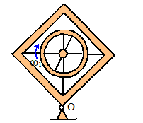
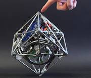 Example 6. The
‘Cubli’ is used to develop control algorithms used to stabilize aircraft
and spacecraft. It consists of a cube
whose attitude can be controlled by spinning a set of reaction wheels inside
the cube.
Example 6. The
‘Cubli’ is used to develop control algorithms used to stabilize aircraft
and spacecraft. It consists of a cube
whose attitude can be controlled by spinning a set of reaction wheels inside
the cube.
This
simplified 1-D version of the device is used to test the algorithm that
stands the cube up on one edge. The
goal of this problem is to do the preliminary design calculations needed to set
up the system.
Idealize the
rectangular frame as four rods with length L
and combined mass M and the spinning
wheel as a ring with radius R and
mass m. The corner at O is supported by a
frictionless bearing.
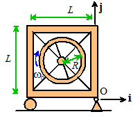 Part 1: Find formulas for the mass moments of inertia of the
frame and the wheel (about the center of the wheel).
Part 1: Find formulas for the mass moments of inertia of the
frame and the wheel (about the center of the wheel).
The ring is easy we can use the formula
The frame is made up of four rods of mass M/4.
The moment of inertia of one rod about its center of mass is . We
need to shift the COM by a distance of L/2
to the center of the frame. The total
mass moment of inertia of the frame is therefore
Part 2: The
frame is at rest and the wheel is spun up (clockwise) to an angular speed . Find
the total angular momentum of the system about the corner at O.
The formula for angular momentum is
Since the frame is not moving only the
second term contributes and we get
 Part 3: Thee wheel is then braked quickly, which causes the
frame to rotate about the corner O at angular speed , while the motor driving the ring spins at
(clockwise) angular speed (note that this is relative to the frame). Write down the angular momentum of the system
about O.
Part 3: Thee wheel is then braked quickly, which causes the
frame to rotate about the corner O at angular speed , while the motor driving the ring spins at
(clockwise) angular speed (note that this is relative to the frame). Write down the angular momentum of the system
about O.
Note that the frame rotates about O so the COM of the ring and frame are
both in circular motion about O. We
know the speed of their COMs are therefore
Use the formula again
We could also use the fixed axis rotation
formula for the frame (using the mass moment of inertia about O) but this would
not work for the ring, because O is not a stationary point on the ring.
 Part 4: Explain why angular momentum is conserved about O
during the braking. Use momentum
conservation to find an equation relating to
Part 4: Explain why angular momentum is conserved about O
during the braking. Use momentum
conservation to find an equation relating to
The external forces acting on the frame and ring together are (1)
gravity and (2) reaction forces at O.
We assume that the speed change of the rotor takes place over a very
short time interval. The force of
gravity is constant and exerts a negligible impulse on the system during this
time interval. The reactions exert a
finite impulse, but if we take moments about O the external angular impulse
about O on the system vanishes. This
means angular momentum must be conserved.
Part 5: For
the special case show that the critical value of required to flip the frame (and ring) into the
stationary vertical configuration is
Energy is conserved as the frame rotates
up onto its edge.
The formula for the kinetic energy of a system
of rigid bodies is
For 2D problems we can replace the last
term by
Assume that the frame is at rest in the
upright state. The total potential and
kinetic energy in the upright state is therefore
In the initial state
Energy conservation gives
For we get
From part 4 we get
6.8.2 Solutions to 3D problems
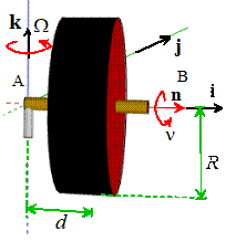 Example 1: The figure shows a wheel spinning on a frictionless
axle. The axle is supported on one side
(at A) by a pivot that allows free rotation in any direction. If the wheel were not spinning, it would
simply swing about A like a pendulum.
But if the angular speed is high enough, the axle remains horizontal,
and the wheel turns slowly about the vertical axis. This behavior is called ‘precession’ and is
a bit mysterious why does spin somehow hold the wheel up? The goal of this example is to explain this,
and to calculate a formula for the rotation rate of the axle.
Example 1: The figure shows a wheel spinning on a frictionless
axle. The axle is supported on one side
(at A) by a pivot that allows free rotation in any direction. If the wheel were not spinning, it would
simply swing about A like a pendulum.
But if the angular speed is high enough, the axle remains horizontal,
and the wheel turns slowly about the vertical axis. This behavior is called ‘precession’ and is
a bit mysterious why does spin somehow hold the wheel up? The goal of this example is to explain this,
and to calculate a formula for the rotation rate of the axle.
We
will do this by showing that steady precession satisfies all the equations of
motion.
1.1
Let n be a unit vector parallel to
the axle. Consider the disk at the
instant when , and assume that
·
the disk spins at
constant rate about the axle at radians per second,
·
the disk rotates
slowly at constant rate about k at radians per second
Find the angular velocity and
angular acceleration at the instant shown in the figure
The
angular velocity is easy we just add the two vectors:
The angular acceleration is harder. Both and are constant.
But this does not mean that the angular velocity vector is constant, because the axle is rotating about the k axis.
The direction of the angular
velocity is changing, even though the magnitude is not. We can calculate the rate of change of n by using the rigid body formula
If
we choose A and B to be a unit distance apart, then and therefore
We
can now calculate the angular acceleration
1.2 Find a formula for the
acceleration of the center of mass of the disk
We
can use the rigid body formula
A
quicker way is to notice that the COM is in circular motion around A and use
the circular motion formula, with the same result.
1.3 Draw a free body diagram
showing the forces acting on the wheel
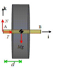
1.3 Write down the equations
of translational and rotational motion for the disk
Working through the cross
products and the matrix-vector products we get
We see that steady precession
can indeed satisfy all the equations of motion.
Moreover, for a disk (or any solid of revolution) , so we can calculate the precession rate
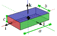 Example 2: The prism shown
in the figure floats in space (no gravity).
At time t=0 its faces are perpendicular to the i,j,k axes as shown. It is then given an initial angular velocity
with (i.e. we set the body spinning about the k axis, but give it a very small
disturbance) . Investigate the nature
of the subsequent motion, with both hand calculations and by writing a MATLAB
script that will animate the motion of the prism.
Example 2: The prism shown
in the figure floats in space (no gravity).
At time t=0 its faces are perpendicular to the i,j,k axes as shown. It is then given an initial angular velocity
with (i.e. we set the body spinning about the k axis, but give it a very small
disturbance) . Investigate the nature
of the subsequent motion, with both hand calculations and by writing a MATLAB
script that will animate the motion of the prism.
No
forces or moments act on the prism. We
can use the equations of motion
The angular momentum equation
can be written out explicitly
(we
could substitute values for in terms of a,b,c and M but it is
clearer to leave them) Expanding out the matrix products and cross product
gives
At
time t=0 is zero and is small.
They might increase, but we will only consider behavior while they
remain small. In this case is extremely small so we can assume . We
can then decouple the first two equations like this:
- Differentiate the second equation with respect to time
- Now we can substitute for using the first equation, and divide by
This is an equation of the
form
We recognize this as an
undamped vibration equation (case I or case II from our table of
solutions). Its solution depends on the
sign of :
- For the solution is where A,
B are constants. This
is stable motion - remains small.
- For the solution is . This
is unstable motion - will become very large.
The sign of is determined by the product . There are three possible cases:
- is greater than (the k
axis has the maximum inertia).
Motion is stable
- is less than (the k
axis has the minimum inertia).
Motion is stable
- is between . Motion
is unstable.
We
can learn more about the motion by using MATLAB to solve the equations of
motion for us. Since there is no motion
of the center of mass, we only need to consider rotational motion. We know that we can describe the orientation
of the prism by the rotation tensor R
and its rate of change of orientation by the angular velocity . The
orientation and angular velocity are governed by the differential equations
where
is the rotated inertia tensor for the block,
and W is the spin tensor
We
need to set up the MATLAB ‘ode’ solver to calculate R and as functions of time by integrating these
equations.
We
can store the unknown rotation matrix and the angular velocity vector in a
MATLAB vector:
We
need to write a MATLAB function that will calculate the time derivatives of
this vector, given its current value.
The calculation involves the following steps:
(1)
Assemble the
vectors and the rotation tensor R from the Matlab solution vector w. Matlab has a useful
function that will automatically convert a matrix to a vector, and vice-versa. For example, (a 3x3 matrix) can be converted to w (a 1x9 column vector) using
w
= reshape(transpose(R),[9,1]))
To
transform w (as a column vector)
back to R, you can use
R
= transpose(reshape(w,[3,3]))
(2) Calculate the spin tensor W
(3) Calculate the rotated inertia tensor (Matlab will multiply the matrices for us)
(4) Solve the equations for the angular acceleration
(5) Calculate
(6) Assemble the matlab vector
This
sounds complicated but actually MATLAB is great at doing this sort of
calculation efficiently. Here’s a
function:
function
dwdt = rigid_body_eom(t,w)
Rvec = w(1:9); %
Rotation matrix, stored as a vector
omega = w(10:12); % Angular velocity
R = transpose(reshape(Rvec,[3,3]));
II = R*I0*transpose(R); %Current inertia tensor, in fixed coord system
W = [0,-omega(3),omega(2);omega(3),0,-omega(1);-omega(2),omega(1),0];
alpha = -II\(cross(omega,II*omega)); % Angular accel
Rdot = W*R; %
Rate of change of rotation matrix
Rdotvec = reshape(transpose(Rdot),[9,1]);
dwdt = [Rdotvec;alpha];
end
We
just need to set up ode45 to integrate (numerically) the differential equation:
omega0 = [0.,0.01,1]; % Initial angular velocity
a = [4,1,2]; % Dimensions (a,b,c) of the prism
time = 20;
initial_w =
[1;0;0;0;1;0;0;0;1;transpose(omega0(1:3))];
I0 =
[a(2)^2+a(3)^2,0,0;0,a(1)^2+a(3)^2,0;0,0,a(1)^2+a(2)^2];
options = odeset('RelTol',0.00000001);
sol = ode45(@(t,w)
rigid_body_eom(t,w,I0),[0,time],initial_w,options);
animate_rigid_body(sol,a,[0,time])
You
can download the full script here.
The
figures below show animations of the predicted behavior for the three possible
types of behavior
|
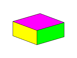
is the maximum inertia rotation is stable
|
|
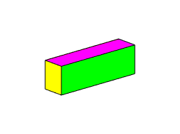
is the intermediate inertia rotation is unstable (the block tumbles)
|
|
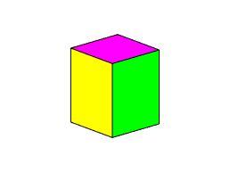
is the smallest inertia rotation is stable
|