
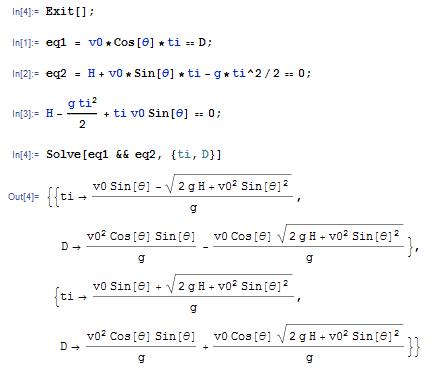
3.3 Deriving and solving equations of motion for systems of particles
We next turn to the more difficult problem of predicting the motion of a system that is subjected to a set of forces.
3.3.1 General procedure for deriving and solving equations of motion for systems of particles
It is very straightforward to analyze the motion of systems of particles. You should always use the following procedure
1. Introduce a set of variables
that can describe the motion of the system.
Don’t worry if this sounds vague it will be clear what this means when we solve
specific examples.
2. Write down the position vector of each particle in the system in terms of these variables
3. Differentiate the position vector(s), to calculate the velocity and acceleration of each particle in terms of your variables;
4. Draw a free body diagram showing the forces acting on each particle. You may need to introduce variables to describe reaction forces. Write down the resultant force vector.
5. Write down for each particle. This will generate up to 3 equations of
motion (one for each vector component) for each particle.
6. If you wish, you can eliminate
any unknown reaction forces from you can have MATLAB calculate the reactions
for you. The result will be a set of differential equations for the variables
defined in step (1)
7. If you find you have fewer equations than unknown variables, you should look for any constraints that restrict the motion of the particles. The constraints must be expressed in terms of the unknown accelerations.
8. Identify the initial conditions for the variables defined in (1). These are usually the values of the unknown variables, their time derivatives, at time t=0. If you happen to know the values of the variables at some other instant in time, you can use that too. If you don’t know their values at all, you should just introduce new (unknown) variables to denote the initial conditions.
9. Solve the differential equations, subject to the initial conditions.
Steps (3) (6) and (8) can usually be done on the computer, so you don’t actually have to do much calculus or math.
Sometimes, you can avoid solving the equations of
motion completely, by using conservation
laws conservation of energy, or conservation of
momentum
to calculate quantities of interest. These short-cuts will be discussed in the
next chapter.
3.2.2 Simple examples of equations of motion and their solutions
The general process described in the preceding section can be illustrated using simple examples. In this section, we derive equations of motion for a number of simple systems, and find their solutions.
The purpose of these examples is to illustrate the straightforward, step-by-step procedure for analyzing motion in a system. Although we solve several problems of practical interest, we will simply set up and solve the equations of motion with some arbitrary values for system parameter, and won’t attempt to explore their behavior in detail. More detailed discussions of the behavior of dynamical systems will follow in later chapters.
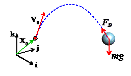
Example 1: Trajectory of a particle near the earth’s surface (no air resistance)
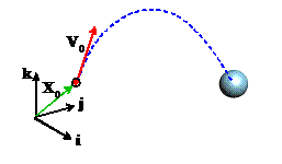
At time t=0,
a projectile with mass m is launched from a position with
initial velocity vector
. Calculate its trajectory as a function of
time.
1.
Introduce variables to describe the
motion: We can simply use the Cartesian coordinates of the
particle
2. Write down the position vector in
terms of these variables:
3. Differentiate the position vector with respect to time to find the acceleration. For this example, this is trivial
4.
Draw a free body diagram. The only force acting on the particle is
gravity the free body diagram is shown in the figure. The force vector follows as
.
5.
Write down
The vector equation actually represents three separate differential equations of motion
6.
Eliminate reactions this is not needed in this example.
7.
Identify initial conditions. The initial conditions were given in this
problem we have that
8. Solve the equations of motion. In general we will use MAPLE or matlab to do the rather tedious algebra necessary to solve the equations of motion. Here, however, we will integrate the equations by hand, just to show that there is no magic in MAPLE.
The equations of motion are
It is a bit easier to see how to solve these if we define
The equation of motion can
be re-written in terms of as
We can separate variables and integrate, using the initial conditions as limits of integration
Now we can re-write the velocity components in terms of (x,y,z) as
Again, we can separate variables and integrate
so the position and velocity vectors are
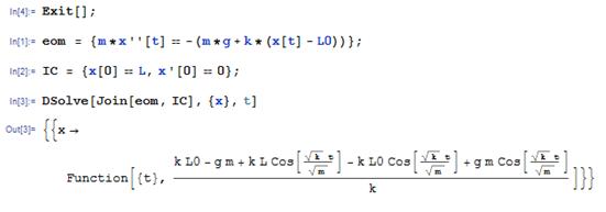
Here’s how to integrate the equations of motion using the `DSolve’ function in Mathematica
Applications of trajectory problems: It is traditional in elementary physics and dynamics courses to solve vast numbers of problems involving particle trajectories. These invariably involve being given some information about the trajectory, which you must then use to work out something else. These problems are all somewhat tedious, but we will show a couple of examples to uphold the fine traditions of a 19th century education.
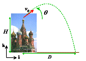 Estimate how far you could throw a stone from
the top of the Kremlin palace.
Estimate how far you could throw a stone from
the top of the Kremlin palace.
Note that
1. The horizontal and vertical components of velocity at time t=0 follow as
2.
The components of
the position of the particle at time t=0
are
3. The trajectory of the particle follows as
4.
When the particle
hits the ground, its position vector is . This must be on the trajectory, so
where
is the time of impact.
5.
The two
components of this vector equation gives us two equations for the two unknowns ,
which can be solved
Only the second solution in
this list is relevant the first has a negative impact time.
For a rough estimate of the distance we can use the following numbers
1.
Height of Kremlin
palace 71m
2. Throwing velocity maybe 25mph?
(pretty pathetic, I know - you can probably do better, especially if you
are on the baseball team).
3.
Throwing angle 45 degrees.
Substituting numbers gives 36m (118ft).
If you want to go wild, you
can maximize D with respect to ,
but this won’t improve your estimate much.
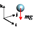
 Silicon nanoparticles with radius 20nm are in thermal motion near a flat
surface. At the surface, they have an
average velocity
Silicon nanoparticles with radius 20nm are in thermal motion near a flat
surface. At the surface, they have an
average velocity ,
where m is their mass, T is the temperature
and k=1.3806503 × 10⁻²³ is the Boltzmann
constant. Estimate the maximum height above the surface that a typical particle
can reach during its thermal motion, assuming that the only force acting on the
particles is gravity
1. The particle will reach its maximum height if it happens to be traveling vertically, and does not collide with any other particles.
2.
At time t=0 such a particle has position and velocity
3. For time t>0 the position vector of the particle follows as
Its velocity is
4. When the particle reaches its maximum height, its
velocity must be equal to zero (if you don’t see this by visualizing the motion
of the particle, you can use the mathematical statement that if is a maximum, then
).
Therefore, at the instant of maximum height
5.
This shows
that the instant of max height occurs at time
6. Substituting this time back into the position vector shows that the position vector at max height is
7. Si has a density of about 2330 kg/m^3. At room
temperature (293K) we find that the distance is surprisingly large: 10mm or
so. Gravity is a very weak force at the nano-scale
surface forces acting between the particles,
and the particles and the surface, are much larger.
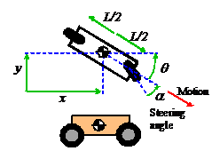
Example 2: Free vibration of a suspension system.
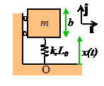
A
vehicle suspension can be idealized as a mass m supported by a spring. The
spring has stiffness k and
un-stretched length . To test the suspension, the vehicle is
constrained to move vertically, as shown in the figure. It is set in motion by
stretching the spring to a length
and then releasing it (from rest). Find an expression for the motion of the
vehicle after it is released.
As
an aside, it is worth noting that a particle idealization is usually too crude
to model a vehicle a rigid body approximation is much
better. In this case, however, we assume
that the vehicle does not rotate. Under these conditions the equations of
motion for a rigid body reduce to
and
,
and we shall find that we can analyze the system as if it were a particle.
1. Introduce
variables to describe the motion: The length of the spring is a
convenient way to describe motion.
2. Write down the position vector in terms of these variables: We can take the origin at O as shown in the figure. The position vector of the center of mass of the block is then
3. Differentiate the position vector with respect to time to find the acceleration. For this example, this is trivial
 4. Draw a free body diagram.
The free body diagram is shown in the figure: the mass is subjected to
the following forces
4. Draw a free body diagram.
The free body diagram is shown in the figure: the mass is subjected to
the following forces
· Gravity, acting at the center of mass of the vehicle
· The force due to the spring
· Reaction forces at each of the rollers that force the vehicle to move vertically.
Recall the spring force law, which says that the forces exerted by a spring act parallel to its length, tend to shorten the spring, and are proportional to the difference between the length of the spring and its un-stretched length.
5.
Write down
The i and j components give two scalar equations of motion
6.
Eliminate reactions this is not needed in this example.
7.
Identify initial conditions. The initial conditions were given in this
problem at time t=0,
we know that
and
8. Solve the equations of motion. Again, we will first integrate the equations of motion by hand, and then repeat the calculation with MAPLE. The equation of motion is
We can re-write this in terms of
This gives
We can separate variables and integrate
Don’t worry if the last
line looks mysterious writing the solution in this form just makes
the algebra a bit simpler. We can now
integrate the velocity to find x
The integral on the left can be evaluated using the substitution
so that
Here’s the Mathematica solution (unfortunately the output format of mathematical is not designed for humans to read)
It doesn’t quite look the
same as the hand calculation but of course
so they really are the same.
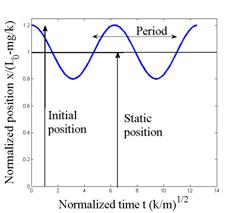 The solution is plotted in the figure. The behavior of vibrating systems will be
discussed in more detail later in this course, but it is worth noting some
features of the solution:
The solution is plotted in the figure. The behavior of vibrating systems will be
discussed in more detail later in this course, but it is worth noting some
features of the solution:
1. The average position of the mass is . Here, mg/k
is the static deflection of the
spring i.e. the deflection of the spring due to the weight of the vehicle
(without motion). This means that the car vibrates symmetrically about its
static deflection.
2.
The amplitude of vibration is . This corresponds to the distance of the mass
above its average position at time t=0.
3.
The period of oscillation (the time taken for
one complete cycle of vibration) is
4.
The frequency of oscillation (the number of
cycles per second) is (note f=1/T). Frequency is also sometimes quoted as angular frequency, which is related to f by
. Angular frequency is in radians per second.
An
interesting feature of these results is that the static deflection is related
to the frequency of oscillation - so if you measure the static deflection ,
you can calculate the (angular) vibration frequency as
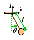
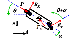
Example 3: Silly FE exam problem
 This example shows how polar
coordinates can be used to analyze motion.
This example shows how polar
coordinates can be used to analyze motion.
The rod shown in the picture rotates at constant
angular speed in the horizontal plane.
The interface between block and rod has friction coefficient . The rod pushes a block of mass m, which starts at r=0 with radial speed V. Find an expression for r(t).
1. Introduce variables to describe the motion the polar coordinates
work for this problem
2. Write down the position vector and differentiate to
find acceleration we don’t need to do this
we can just write down the standard result for
polar coordinates
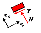
3. Draw a free body diagram shown in the figure
note that it is important to draw the friction
force in the correct direction. The
block will slide radially outwards, and friction opposes the slip.
4. Write down Newton’s law
5. Eliminate reactions
F=ma gives two
equations for N and T.
A third one comes from the friction law
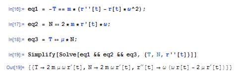
The last solution can be rearranged into an equation of motion for r
6. Identify initial conditions Here, r=0 dr/dt=V at time t=0.
7. Solve the equation: If you’ve taken AM33 you will know how to solve this equation… But if not, or you are lazy, you can use Mathematica to solve it for you.
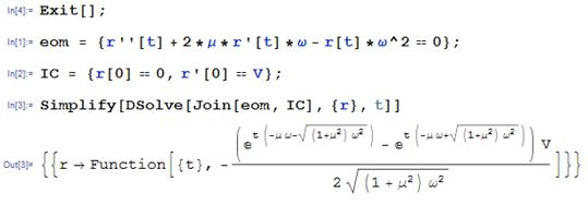
(if you are very comfortable with Mathematica, you can have Mathematica solve the three
equations and the ODE together but the syntax to do this is very confusing to
read, so we use the clearest approach here)
This can be simplified slightly by hand:
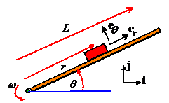
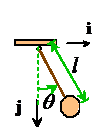
 Example 4: Motion of a pendulum (R-rated version)
A pendulum is a ubiquitous engineering system. You are, of course, familiar with how a pendulum can be used to measure time. But it’s used for a variety of other scientific applications. For example, Professor Crisco’s lab uses pendulum to measure properties of human joints, see
Crisco Joseph J; Fujita Lindsey; Spenciner David B, ‘The dynamic flexion/extension properties of the lumbar spine in vitro using a novel pendulum system.’ Journal of biomechanics 2007;40(12):2767-73
In this example, we will work through the basic problem of deriving and solving the equations of motion for a pendulum, neglecting air resistance.
1.
Introduce variables to describe
motion: The angle shown in the figure is a convenient variable.
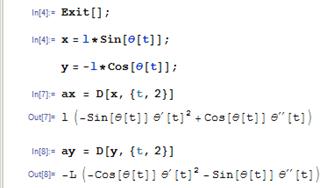
2. Write down the position vector as a function of the variables We introduce a Cartesian coordinate system with origin at O, as shown in the picture.
Elementary geometry shows
that
Note
that we have assumed that the cable remains straight this will be true as long as the internal
force in the cable is tensile. If
calculations predict that the internal force is compressive, this assumption is
wrong. But there is no way to check the
assumption at this point so we simply proceed, and check the answer at the end
3. Differentiate the position vector to find the acceleration: The computer makes this painless.
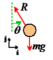
4. The free body diagram is shown in the figure. The force exerted by the cable on the particle is introduced as an unknown reaction force. The force vector is
5.
Equating the i and j components gives two equations for the two unknowns
6.
Eliminate
the reaction forces. In this problem, it is helpful to eliminate
the unknown reaction force R. You can do this on the computer if you like,
but in this case it is simpler to do this by hand. You can simply multiply the first equation by
and the second equation by
and then add them. This yields
7.
Identify
initial conditions. Some calculations are necessary to determine the
initial conditions in this problem. We
are given that at time t=0,
and the horizontal velocity is
at time t=0,
but to solve the equation of motion, we need the value of
. We can find the relationship we need by
differentiating the position vector to find the velocity
Setting and
at t=0
shows that
so
8.
Solve
the equations of motion This
equation of motion is too difficult for Mathematica (it can come close to
getting a solution if you don’t specify any initial conditions) but actually
the solution does exist and is very well known this is a classic problem in mathematical
physics. With initial conditions
the solution is
The first solution describes swinging motion of the pendulum, while the second solution describes the motion that occurs if you push the pendulum so hard that it whirls around on the pivot. The equations may look scary, but you can simply use MAPLE to calculate and plot them.
- In the first equation,
is a special function called the `sin amplitude.’ You can think of it as a sort of trig function for adultsin fact for k=0,and we recover the PG version. You can compute it in Mathematica using JacobiSN[x,k]
- Similarly, is a function called the `Amplitude.’ You can calculate it in MAPLE using ‘JacobiAmplitude[x,k]’ In Mathematica, the am function has range, so the solution predicts that as the pendulum whirls around the pivot, the angleincreases from 0 to, then jumps to, increases toagain, and so on.
You
might have solved the pendulum problem already in an elementary physics course,
and might remember a different solution.
This is because you probably only derived an approximate solution, by assuming that the angle remains small. This occurs when the initial velocity
satisfies
, in which case the solution can be approximated by
3.3.3 Numerical solutions to equations of motion using MATLAB
In the preceding section, we were able to solve all
our equations of motion exactly, and hence to find formulas that describe the motion of the system. This should give you a warm and fuzzy feeling
it appears that with very little work, you can
predict everything about the motion of the system. You may even have visions of running a
consulting business from your yacht in the Caribbean, with nothing more than your
chef, your masseur (or masseuse) and a laptop with a copy of Mathematica
Unfortunately real life is not so simple. Equations of motion for most engineering systems cannot be solved exactly. Even very simple problems, such as calculating the effects of air resistance on the trajectory of a particle, cannot be solved exactly.
For
nearly all practical problems, the equations of motion need to be solved numerically, by using a computer to calculate
values for the position, velocity and acceleration of the system as functions
of time. Vast numbers of computer programs have been written for this purpose some focus on very specialized applications,
such as calculating orbits for spacecraft (STK); calculating motion of atoms in
a material (LAMMPS); solving fluid flow problems (e.g. fluent, CFDRC); or
analyzing deformation in solids (e.g. ABAQUS, ANSYS, NASTRAN, DYNA); others are
more general purpose equation solving programs.
In this course we will use a general purpose program called MATLAB, which is widely used in all engineering applications. You should complete the MATLAB tutorial before proceeding any further.
In the remainder of this section, we provide a number of examples that illustrate how MATLAB can be used to solve dynamics problems. Each example illustrates one or more important technique for setting up or solving equations of motion.
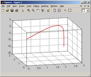
Example 1: Trajectory of a particle near the earth’s surface (with air resistance)
 As a simple example we set
up MATLAB to solve the particle trajectory problem discussed in the preceding
section. We will extend the calculation
to account for the effects of air resistance, however. We will assume that our projectile is
spherical, with diameter D, and we
will assume that there is no wind. You
may find it helpful to review the discussion of aerodynamic drag forces in
Section 2.1.7 before proceeding with this example.
As a simple example we set
up MATLAB to solve the particle trajectory problem discussed in the preceding
section. We will extend the calculation
to account for the effects of air resistance, however. We will assume that our projectile is
spherical, with diameter D, and we
will assume that there is no wind. You
may find it helpful to review the discussion of aerodynamic drag forces in
Section 2.1.7 before proceeding with this example.
1. Introduce
variables to describe the motion: We can simply use the Cartesian
coordinates of the particle
2. Write down the position vector in
terms of these variables:
3. Differentiate the position vector with respect to time to find the acceleration. Simple calculus gives
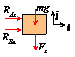
4. Draw a free body diagram. The particle is now subjected to two forces, as shown in the picture.
Gravity
as always we have
.
Air resistance.
The
magnitude of the air drag force is given
by ,
where
·
is the air density,
·
is the drag coefficient,
· D is the projectile’s diameter, and
·
is the magnitude of the projectile’s velocity
relative to the air. Since we assumed the air is stationary, V is simply the magnitude of the
particle’s velocity, i.e.
The Direction
of the air drag force is always opposite to the direction of motion of the
projectile through the air. In this case
the air is stationary, so the drag force is simply opposite to the direction of
the particle’s velocity. Note that is a unit vector parallel to the particle’s
velocity. The drag force vector is
therefore
The total force vector is therefore
5.
Write down
It is helpful to simplify
the equation by defining a specific drag
coefficient ,
so that
The vector equation actually represents three separate differential equations of motion
6.
Eliminate reactions this is not needed in this example.
7. Identify initial conditions. The initial conditions were given in this problem - we have that
8. Solve
the equations of motion. We
can’t use the magic ‘dsolve’ command in MAPLE to solve this equation it has no known exact solution. So instead, we use MATLAB to generate a
numerical solution.
This takes two steps. First, we must turn the equations of motion
into a form that MATLAB can use. This
means we must convert the equations into first-order vector valued differential
equation of the general form . Then, we must write a MATLAB script to
integrate the equations of motion.
Converting the equations of motion: We can’t
solve directly for (x,y,z), because
these variables get differentiated more than once with respect to time. To fix this, we introduce the time derivatives of (x,y,z) as new unknown variables. In other words, we will solve for ,
where
These definitions are three new equations of motion relating our unknown variables. In addition, we can re-write our original equations of motion as
So, expressed as a vector valued differential equation, our equations of motion are
MATLAB script. The procedure for solving these equations is discussed in the MATLAB tutorial. A basic MATLAB script is listed below.
function trajectory_3d
% Function to plot trajectory of a projectile
% launched from position X0 with velocity V0
% with specific air drag coefficient c
% stop_time specifies the end of the calculation
g = 9.81; % gravitational accel
c=0.5; % The constant c
X0=0; Y0=0; Z0=0; % The initial position
VX0=10; VY0=10; VZ0=20;
stop_time = 5;
initial_w = [X0,Y0,Z0,VX0,VY0,VZ0]; % The solution at t=0
[times,sols] = ode45(@eom,[0,stop_time],initial_w);
plot3(sols(:,1),sols(:,2),sols(:,3)) % Plot the trajectory
function dwdt = eom(t,w)
% Variables stored as follows w = [x,y,z,vx,vy,vz]
% i.e. x = w(1), y=w(2), z=w(3), etc
x = w(1); y=w(2); z=w(3);
vx = w(4); vy = w(5); vz = w(6);
vmag = sqrt(vx^2+vy^2+vz^2);
dxdt = vx; dydt = vy; dzdt = vz;
dvxdt = -c*vmag*vx;
dvydt = -c*vmag*vy;
dvzdt = -c*vmag*vz-g;
dwdt = [dxdt;dydt;dzdt;dvxdt;dvydt;dvzdt];
end
end
This produces a plot that looks like this (the plot’s been edited to add the grid,etc)
 Example 2:
Simple satellite orbit calculation
Example 2:
Simple satellite orbit calculation
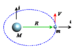
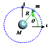
The figure shows satellite with mass m orbiting a planet with mass M.
At time t=0 the satellite has
position vector and velocity vector
. The planet’s motion may be neglected (this is
accurate as long as M>>m). Calculate
and plot the orbit of the satellite.
1. Introduce variables to describe the motion: We will use the (x,y) coordinates of the satellite.
2. Write down the position vector in
terms of these variables:
3. Differentiate the position vector with respect to time to find the acceleration.
4. Draw a free body diagram. The satellite is subjected to a gravitational force.
The
magnitude of the force is ,
where
·
is the gravitational constant, and
·
is the distance between the planet and the
satellite
The
direction of the force is always towards the origin: is
therefore a unit vector parallel to the direction of the force. The total force acting on the satellite is
therefore
5.
Write down
The vector equation represents two separate differential equations of motion
6.
Eliminate reactions this is not needed in this example.
7. Identify initial conditions. The initial conditions were given in this problem - we have that
8. Solve the equations of motion. We follow the usual procedure: (i) convert the equations into MATLAB form; and (ii) code a MATLAB script to solve them.
Converting the equations of motion: We introduce
the time derivatives of (x,y) as new
unknown variables. In other words, we
will solve for ,
where
These definitions are new equations of motion relating our unknown variables. In addition, we can re-write our original equations of motion as
So, expressed as a vector valued differential equation, our equations of motion are
Matlab script: Here’s a simple script to solve these equations.
function satellite_orbit
% Function to plot orbit of a satellite
% launched from position (R,0) with velocity (0,V)
GM=1;
R=1;
V=1;
Time=100;
w0 = [R,0,0,V]; % Initial conditions
[t_values,w_values] = ode45(@odefunc,[0,time],w0);
plot(w_values(:,1),w_values(:,2))
function dwdt = odefunc(t,w)
x=w(1);
y=w(2); vx=w(3); vy=w(4);
r = sqrt(x^2+y^2);
dwdt = [vx;vy;-GM*x/r^3;-GM*y/r^3];
end
end
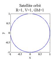
Running the script produces the result shown (the plot was annotated by hand)
Do we believe this result? It is a bit surprising the satellite seems to be spiraling in towards
the planet. Most satellites don’t do
this
so the result is a bit suspicious. The First Law of Scientific Computing states
that ` if a computer simulation predicts
a result that surprises you, it is probably wrong.’
So how can we test our computation? There are two good tests:
1. Look for any features in the simulation that you can predict without computation, and compare your predictions with those of the computer.
2. Try to find a special choice of system parameters for which you can derive an exact solution to your problem, and compare your result with the computer
We can use both these checks here.
1.
Conserved quantities For this particular problem, we
know that (i) the total energy of the system should be constant; and (ii) the
angular momentum of the system about the planet should be constant (these
conservation laws will be discussed in the next chapter for now, just take this as given). The total energy of the system consists of
the potential energy and kinetic energy of the satellite, and can be calculated
from the formula
The total angular momentum of the satellite (about the origin) can be calculated from the formula
(If you don’t know these formulas, don’t
panic we will discuss energy and angular momentum in
the next part of the course)
We
can have MATLAB plot E/m and ,
and see if these are really conserved. The energy and momentum can be calculated by
adding these lines to the MATLAB script
for i =1:length(t)
r = sqrt(w_values(i,1)^2 + w_values(i,2)^2)
vmag = sqrt(w_values(i,1)^2 + w_values(i,2)^2)
energy(i) = -GM/r + vmag^2/2;
angularm(i) = w_values(i,1)*w_values(i,4)-w_values(i,2)*w_values(i,3);
end
You can then plot the results (e.g. plot(t_values,energy)). The results are shown below.
These
results look really bad neither energy, nor angular momentum, are conserved
in the simulation. Something is clearly
very badly wrong.
 Comparison to exact solution: It is not always possible to
find a convenient exact solution, but in this case, we might guess that some
special initial conditions could set the satellite moving on a circular path. A circular path might be simple enough to
analyze by hand. So let’s assume that
the path is circular, and try to find the necessary initial conditions. If you
still remember the circular motion formulas, you could use them to do
this. But only morons use formulas
Comparison to exact solution: It is not always possible to
find a convenient exact solution, but in this case, we might guess that some
special initial conditions could set the satellite moving on a circular path. A circular path might be simple enough to
analyze by hand. So let’s assume that
the path is circular, and try to find the necessary initial conditions. If you
still remember the circular motion formulas, you could use them to do
this. But only morons use formulas here we will derive the solution from scratch.
Note that, for a circular path
(a) the particle’s radius r=constant. In fact, we know r=R, from the position at time t=0.
(b) The satellite must move
at constant speed, and the angle must increase linearly with time, i.e.
where
is a constant (see section 3.1.3 to review
motion at constant speed around a circle).
With this information we can solve the equations of motion. Recall that the position, velocity and acceleration vectors for a particle traveling at constant speed around a circle are
We
know that from the initial conditions, and
is constant. This tells us that
Finally, we can substitute
this into
Both components of the equation of motion are satisfied if we choose
So, if we choose initial
values of satisfying this equation, the orbit will be
circular. In fact, our original choice,
should have given a circular orbit. It did not.
Again, this means our computer generated solution is totally wrong.
 Fixing the
problem: In general, when computer predictions are
suspect, we need to check the following
Fixing the
problem: In general, when computer predictions are
suspect, we need to check the following
1. Is there an error in our MATLAB program? This is nearly always the cause of the problem. In this case, however, the program is correct (it’s too simple to get wrong, even for me).
2. There may be something wrong with our equations of motion (because we made a mistake in the derivation). This would not explain the discrepancy between the circular orbit we predict and the simulation, since we used the same equations in both cases.
3. Is the MATLAB solution sufficiently accurate? Remember that by default the ODE solver tries to give a solution that has 0.1% error. This may not be good enough. So we can try solving the problem again, but with better accuracy. We can do this by modifying the MATLAB call to the equation solver as follows
options = odeset('RelTol',0.00001);
[t_values,w_vlues] = ode45(@odefunc,[0,time],w0,options);
- Is there some feature of the equation of motion that makes them especially difficult to solve? In this case we might have to try a different equation solver, or try a different way to set up the problem.
The figure on the right shows the orbit
predicted with the better accuracy. You
can see there is no longer any problem the orbit is perfectly circular. The figures below plot the energy and
angular momentum predicted by the computer.
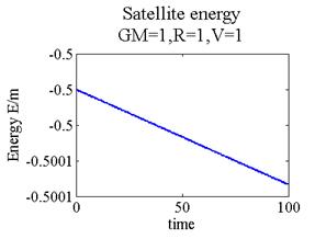
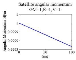
There is a small change in energy and angular momentum but the rate of change has been reduced dramatically. We can make the error smaller still by using improving the tolerances further, if this is needed. But the changes in energy and angular momentum are only of order 0.01% over a large number of orbits: this would be sufficiently accurate for most practical applications.
Most ODE
solvers are purposely designed to lose a small amount of energy as the
simulation proceeds, because this helps to make them more stable. But in some applications this is unacceptable
for example in a molecular dynamic simulation
where we are trying to predict the entropic response of a polymer, or a free
vibration problem where we need to run the simulation for an extended period of
time. There are special ODE solvers that
will conserve energy exactly.
Example 3: Earthquake response of a 2-storey building
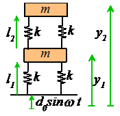 The figure shows a very
simple idealization of a 2-storey building.
The roof and second floor are idealized as blocks with mass m.
They are supported by structural columns, which can be idealized as springs
with stiffness k and unstretched
length L. At time t=0
the floors are at rest and the columns have lengths
The figure shows a very
simple idealization of a 2-storey building.
The roof and second floor are idealized as blocks with mass m.
They are supported by structural columns, which can be idealized as springs
with stiffness k and unstretched
length L. At time t=0
the floors are at rest and the columns have lengths (can you show this?). We will neglect the thickness of the floors
themselves, to keep things simple.
For
time t>0, an earthquake makes the
ground vibrate vertically. The ground motion can be described using the
equation . Horizontal motion may be neglected. Our goal
is to calculate the motion of the first and second floor of the building.
It is worth noting a few points about this problem:
1. You may be skeptical that the floor of a building can
be idealized as a particle (then again, maybe you couldn’t care less…). If so, you are right it certainly is not a `small’ object. However, because the floors move vertically
without rotation, the rigid body equations of motion simply reduce to
and M=0,
where the moments are taken about the center of mass of the block. The floors behave as though they are particles,
even though they are very large.
2. Real earthquakes involve predominantly horizontal, not vertical motion of the ground. In addition, structural columns resist extensional loading much more strongly than transverse loading. So we should really be analyzing horizontal motion of the building rather than vertical motion. However, the free body diagrams for horizontal motion are messy (see if you can draw them) and the equations of motion for vertical and horizontal motion turn out to be the same, so we consider vertical motion to keep things simple.
3. This problem could be solved analytically (e.g. using
the `dsolve’ feature of MAPLE) a numerical solution is not necessary. Try this for yourself.
1. Introduce
variables to describe the motion: We will use the height of each floor as the variables.
2. Write down the position vector in terms of these variables: We now have to worry about two masses, and must write down the position vector of both
Note that we must measure the position of each mass from a fixed point.
3. Differentiate the position vector with respect to time to find the acceleration.
4. Draw a free body diagram. We must draw a free body diagram for each mass. The resultant force acting on the bottom and top masses, respectively, are
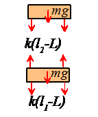
We
will have to find the spring lengths in terms of our coordinates
to solve the problem. Geometry shows that
5.
Write down
This is two equations of
motion we can substitute for
and rearrange them as
6.
Eliminate reactions this is not needed in this example.
7. Identify initial conditions. We know that, at time t=0
8. Solve the equations of motion. We need to (i) reduce the equations to the standard MATLAB form and (ii) write a MATLAB script to solve them.
Converting the equations. We now need
to do two things: (a) remove the second derivatives with respect to time, by
introducing new variables; and (b) rearrange the equations into the form . We remove the derivatives by introducing
as additional unknown variables, in the usual
way. Our equations of motion can then
be expressed as
We can now code MATLAB to solve these equations directly for dy/dt. A script (which plots the position of each floor as a function of time) is shown below.
function building
%
k=100;
m=1;
omega=9;
d=0.1;
L=10;
time=20;
g = 9.81;
w0 = [L-m*g/k,2*L-3*m*g/(2*k),0,0];
[t_values,w_values] = ode45(@eom,[0,time],w0);
plot(t_values,w_values(:,1:2));
function dwdt = eom(t,w)
y1=w(1);
y2=w(2);
v1=w(3);
v2=w(4);
dwdt =
[v1;v2;...
-2*k*(y1-d*sin(omega*t)-L)/m+2*k*(y2-y1-L)/m;...
-g-2*k*(y2-y1-L)/m]
end
end
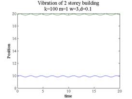
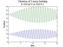
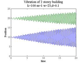
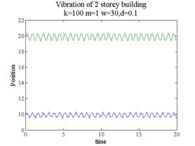
The figures below plot the height of each floor as a function of time, for various earthquake frequencies. For special earthquake frequencies (near the two resonant frequencies of the structure) the building vibrations are very severe. As long as the structure is designed so that its resonant frequencies are well away from the frequency of a typical earthquake, it will be safe.
We will discuss vibrations in much more detail later in this course.
 Example 4:
The dreaded pendulum revisited (apologies…)
Example 4:
The dreaded pendulum revisited (apologies…)
You may have lost interest in pendulum problems by now. Bear with us, however- it is a convenient example that illustrates how to solve problems with constraints.
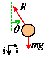
So we re-visit the problem shown in the figure. This time, we will describe the system using (x,y) coordinates of the mass instead of the inclination of the cable.
1. Introduce
variables to describe the motion: We will use the position of the mouse
relative to point O as the variables.
2. Write down the position vector in terms of these variables:
Note that we’ve chosen j to point vertically downwards
3. Differentiate the position vector with respect to time to find the acceleration.
4.
Draw a free body diagram. We
can use the FBD we drew earlier. The
force must now be expressed in terms of x
and y instead of ,
however. Simple trig shows that
The resultant force is therefore
5.
Write down
This is two equations of
motion we can rearrange them as
6. Eliminate
reactions We
could eliminate R if we wanted
but this time we won’t bother. Instead, we will carry R along as an additional unknown, and use MATLAB to calculate
it.
7.
If
there are more unknown variables than equations of motion, look for constraint
equations. We now have three unknowns (x,y,R) but only two equations of motion
(eliminating R in step 6 won’t help in this case we will have two unknowns but
only one equation of motion). So we need
to look for an additional equation somewhere.
The
reason we’re missing an equation is that we took x,y to be arbitrary but of course the mouse has to remain attached
to the cable at all times. This means
that his distance from O is fixed
i.e.
This is the missing equation.
We could, if we wanted, use this equation to eliminate one of our unknown variables (doing the algebra by hand). Instead, however, we will use MATLAB to do this for us. For this purpose, we need to turn the equation into a constraint on the accelerations, instead of the position of the particle. To get such an equation, we can differentiate both sides of the constraint with respect to time
This is now a constraint on the velocity. Differentiating again gives
Again
if you have trouble doing the derivatives, just
use MAPLE (don’t forget to specify that x,
y are functions of time, i.e. enter
them as x(t), y(t) when typing the constraint formula into MAPLE).
[Aside when
I first coded this problem I tried to constrain the velocity of the particle, instead of the acceleration. This doesn’t work (as I should have known),
and produces some rather interesting MATLAB errors
if you are curious, try it and see what
happens. If you are even more curious,
you might like to think about why
you need to constrain accelerations and not velocities.]
7. Identify initial conditions. We know that, at time t=0
8. Solve the equations of motion. We need to (i) reduce the equations to the standard MATLAB form and (ii) write a MATLAB script to solve them.
In the usual way, we introduce as additional unknowns. Our set of unknown
variables is
. The equations of motion, together with the
constraint equation, can be expressed as
This can be expressed as a matrix equation for an unknown
vector
We
can now use MATLAB to solve the equations for the unknown time derivatives ,
together with the reaction force R. Here’s a MATLAB script that integrates the
equations of motion and plots (x,y)
as a function of time. Notice that,
because we don’t need to integrate R
with respect to time, the function ‘eom’ only needs to return
.
function pendulum
g = 9.81;
l=1;
V0=0.1;
time=20;
w0 = [0,l,V0,0]; % Initial conditions
[t_values,w_values] = ode45(@eom,[0,time],w0);
plot(t_values,w_values(:,1:2));
function dwdt = eom(t,w)
% The vector w contains [x,y,vx,vy]
x=w(1);y=w(2);vx=w(3);vy=w(4);
M = eye(5); % This sets up a 5x5 matrix with 1s on all the diags
M(3,5) = (x/m)/sqrt(x^2+y^2);
M(4,5) = (y/m)/sqrt(x^2+y^2);
M(5,3) = x;
M(5,4) = y;
M(5,5) = 0;
f = [vx;vy;0;g;-vx^2-vy^2];
sol = M\f; % This solves the matrix equation M*[dydt,R]=f for [dwdt,R]
dwdt = sol(1:4); % only need to return time derivatives dw/dt
end
end
Final
remarks: In
general, it is best to avoid using constraint equations it makes the problem harder to set up, and
harder for MATLAB to solve. Sometimes they are unavoidable, however
in some cases you might not see how to
identify a suitable set of independent coordinates; and there are some systems
(a rolling wheel is the most common example) for which a set of independent
coordinates do not exist. These are
given the fancy name `non-holonomic systems’
mentioning that you happen to be an expert on
non-holonomic systems during a romantic candle-light dinner is sure to impress
your dates.
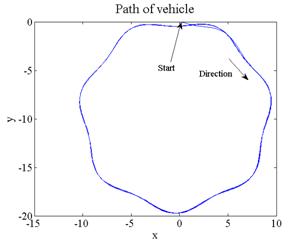
3.3.4 Case Study - Simple model of a vehicle
 As a representative
application of the methods outlined in the preceding section, we will set up
and solve the equations of motion for a very simple idealization of a vehicle. This happens to be an example of a non-holonomic system (sorry we aren’t at
a romantic dinner). Don’t worry if the
model looks rather scary
As a representative
application of the methods outlined in the preceding section, we will set up
and solve the equations of motion for a very simple idealization of a vehicle. This happens to be an example of a non-holonomic system (sorry we aren’t at
a romantic dinner). Don’t worry if the
model looks rather scary this calculation is more advanced than
anything you would be expected to do at this stage of your career… Our goal is to illustrate how the method
we’ve developed in this section can be applied to a real engineering system of
interest. You should be able to follow and understand
the procedure.
The figure shows how the vehicle is idealized. Here are a few remarks:
1. We consider only 2D planar motion of the vehicle
2. For simplicity we assume the vehicle has only two wheels, one at the front and one at the rear. (It’s not a motorcycle, however, because we won’t account for the vehicle leaning around corners)
3. The car is idealized as a particle with mass m supported on a massless chassis with wheelbase L.
4. Aerodynamic drag forces are assumed to act directly on the particle.
5. The most complicated and important part of a vehicle dynamics model is the description of how the wheels interact with the road. Here, we will just assume that
a. The front and rear of the vehicle have to move in a direction perpendicular to each wheel’s axle. Reaction forces must act on each wheel parallel to the axle in order to enforce this constraint (see the FBD).
b. In addition, we assume that
the vehicle has rear-wheel drive. This is modeled as a prescribed force exerted by the ground on the rear wheel,
acting parallel to the rolling direction of the wheel (see the FBD).
c. The front wheel is assumed to roll freely and have
negligible mass this means that the contact force acting on
the wheel must be perpendicular to its rolling direction (see the FBD). The
vehicle is steered by rotating the front wheel through an angle
with respect to the chassis.
This is a vastly over-simplified model of wheel/road
interaction for example, it predicts that the car can
never skid. If you are interested in
extending this calculation to a more realistic model, ask us… We’d be happy to
give you better equations!
1.
Introduce variables to describe the
motion: We will use the (x,y)
coordinates of car and its orientation as the variables.
2. Write down the position vector in
terms of these variables:
3. Differentiate the position vector with respect to time to find the acceleration.
 4. Draw a free body diagram. The vehicle is subjected to (i) a
thrust force P and a lateral reaction
force
4. Draw a free body diagram. The vehicle is subjected to (i) a
thrust force P and a lateral reaction
force acting on the rear wheel, (ii) a lateral
reaction force
acting on the front wheel, and a drag force
acting at the center of mass.
The drag force is related to the vehicle’s velocity by
where c is a drag coefficient. For a more detailed discussion of drag forces see the first example in this section.
The resultant force on the vehicle is
Because we are modeling the motion of the vehicle’s chassis, which can rotate, we must also consider the moments acting on the chassis. You should be able to verify for yourself that the resultant moment of all the forces about the particle is
5.
Write down
This gives two equations of motion; the condition M=0 for the chassis gives one more.
6. Eliminate
reactions It’s easier to eliminate them with MATLAB.
7. If there are more unknown variables than equations of motion, look for constraint equations. This is the hard part of this application. We have two unknown reaction forces, so we need to find two constraint equations that will determine them. These are (i) that the rear of the vehicle must move perpendicular to the axle of the rear wheel; and (ii) the front of the vehicle must move perpendicular to the axle of the front wheel. Consider the rear wheel:
1. Note
that the position vector of the rear wheel is
2. The velocity follows as
3. Note that is a unit vector parallel to the axle of the
rear wheel.
4. For the rear of the vehicle to move perpendicular to
the rear axle, we must have .
This shows that
Similarly, for the front wheel, we can show that
where we have used the trig
formula .
We need to re-write these equations as constraints on the acceleration of the vehicle. To do this, we differentiate both constraints with respect to time, to see that
7. Identify initial conditions: We will assume that the vehicle starts at rest, with
7. Solve the equations of motion. We need to write the equations of motion in a suitable matrix form for MATLAB. We need to eliminate all the second derivatives with respect to time from the equations of motion, by introducing new variables. To do this, we define
as new variables, and then
solve for . We also need to eliminate the unknown
reactions. It is not hard to show that
the equations of motion, in matrix form, are
where
Finally,
we can type these into MATLAB here’s a simple script that solves the
equations of motion and plots the (x,y)
coordinates of the car to show its path, and also plots the speed of the car as
a function of time. The example
simulates a drunk-driver, who steers with steering angle
,
and drives with his or her foot to the floor with P=constant.
function drivemycar
L=1;
m=1;
c=0.1;
time=120;
y0 = [0,0,0,0,0,0];
options = odeset('RelTol',0.00001);
[t_vals,w_vals] = ode45(@eom,[0,time],y0,options);
plot(w_vals(:,1),w_vals(:,2));
function [alpha,dadt,P]=driver(t)
% This function behaves like the driver of the car -
% at time t it returns the steering angle alpha
% dalpha/dt and the driving force P
alpha = 0.1+0.2*sin(t);
dadt = 0.2*cos(t);
P = 0.2;
end
function dwdt = eom(t,w)
% Equations of motion for the vehicle
%
[alpha,dadt,P] = driver(t); % Find out what the driver is doing
M = zeros(8); % This sets up a 8x8 matrix full of zeros
M(1,1) = 1;
M(2,2) = 1;
M(3,3) = 1;
M(4,4) = m;
M(4,7)=-sin(w(3)+alpha);
M(4,8)=-sin(w(3));
M(5,5)=m;
 M(5,7)=-cos(w(3)+alpha);
M(5,8)=-cos(w(3));
M(6,7)=cos(alpha);
M(6,8)=-1;
M(7,4)=sin(w(3));
M(7,5)=cos(w(3));
M(7,6)=L/2;
M(8,4)=sin(w(3)+alpha);
M(8,5)=cos(w(3)+alpha);
M(8,6)=-L*cos(alpha)/2;
v = sqrt(w(4)^2+w(5)^2);
f = [w(4);
w(5);
w(6);
P*cos(w(3))-c*v*w(4);
-P*sin(w(3))-c*v*w(5);
0;
(-cos(w(3))*w(4)+sin(w(3))*w(5))*w(6);
(-cos(w(3)+alpha)*w(4)+sin(w(3)+alpha)*w(5))*(w(6)+dadt)-sin(alpha)*L*w(6)*dadt/2];
sol = M\f; % This solves the matrix equation M*[dwdt,R]=f for [dwdt,R]
dwdt = sol(1:6); % only need to return time derivatives dw/dt
end
end