
5.4 Forced vibration of damped, single degree of freedom, linear spring mass systems.
Finally, we solve the most important vibration problems of all. In engineering practice, we are almost invariably interested in predicting the response of a structure or mechanical system to external forcing. For example, we may need to predict the response of a bridge or tall building to wind loading, earthquakes, or ground vibrations due to traffic. Another typical problem you are likely to encounter is to isolate a sensitive system from vibrations. For example, the suspension of your car is designed to isolate a sensitive system (you) from bumps in the road. Electron microscopes are another example of sensitive instruments that must be isolated from vibrations. Electron microscopes are designed to resolve features a few nanometers in size. If the specimen vibrates with amplitude of only a few nanometers, it will be impossible to see! Great care is taken to isolate this kind of instrument from vibrations. That is one reason they are almost always in the basement of a building: the basement vibrates much less than the floors above.
We will again use a spring-mass system as a model of a real engineering system. As before, the spring-mass system can be thought of as representing a single mode of vibration in a real system, whose natural frequency and damping coefficient coincide with that of our spring-mass system.
We will consider three types of forcing applied to the spring-mass system, as shown below:
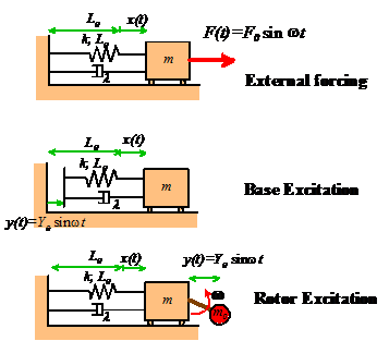
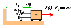
External Forcing models the behavior of a system which has a time varying force acting on it. An example might be an offshore structure subjected to wave loading.
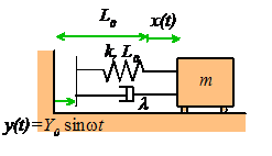
Base Excitation models the behavior of a vibration isolation system. The base of the spring is given a prescribed motion, causing the mass to vibrate. This system can be used to model a vehicle suspension system, or the earthquake response of a structure.
Rotor Excitation models the effect of a rotating machine mounted on a
flexible floor. The crank with small
mass rotates at constant angular velocity, causing
the mass m to vibrate.
Of course, vibrating systems can be excited in other ways as well, but the equations of motion will always reduce to one of the three cases we consider here.
Notice that in each case, we will restrict our analysis to harmonic excitation. For example, the external force applied to the first system is given by
The
force varies harmonically, with amplitude and frequency
.
Similarly, the base motion for the second system is
and
the distance between the small mass and the large mass m for the third system has the same form.
We assume that at time t=0, the initial position and velocity of each system is
In each case, we wish to calculate the displacement of the mass x from its static equilibrium configuration, as a function of time t. It is of particular interest to determine the influence of forcing amplitude and frequency on the motion of the mass.
We follow the same approach to analyze each system: we set up, and solve the equation of motion.
5.4.1 Equations of Motion for Forced Spring Mass Systems
Equation of Motion for External Forcing
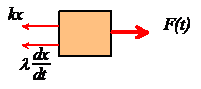 We have no problem setting up and solving equations of
motion by now. First draw a free body
diagram for the system, as show on the right
We have no problem setting up and solving equations of
motion by now. First draw a free body
diagram for the system, as show on the right
Newton’s law of motion gives
Rearrange and susbstitute for F(t)
Check out our list of solutions to standard ODEs. We find that if we set
,
our equation can be reduced to the form
which is on the list.
The (horrible) solution to this equation is given in the list of solutions. We will discuss the solution later, after we have analyzed the other two systems.
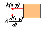
Equation of Motion for Base Excitation
Exactly
the same approach works for this system.
The free body diagram is shown in the figure. Note that the
force in the spring is now k(x-y) because
the length of the spring is . Similarly, the rate of change of length
of the dashpot is d(x-y)/dt.
Newton’s second law then tells us that
Make the following substitutions
and the equation reduces to the standard form
Given the initial conditions
and the base motion
we can look up the solution in our handy list of solutions to ODEs.
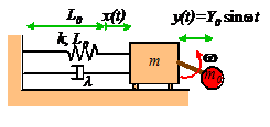
Equation of motion for Rotor Excitation
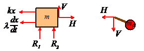
Finally, we will derive the equation of motion for the third case. Free body diagrams are shown below for both the rotor and the mass
Note that the horizontal
acceleration of the mass is
Hence, applying Newton’s second law in the horizontal direction for both masses:
Add these two equations to eliminate H and rearrange
To arrange this into standard form, make the following substitutions
whereupon the equation of motion reduces to
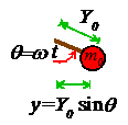
Finally, look at the
picture to convince yourself that if the crank rotates with angular velocity ,
then
where is the length of the crank.
The solution can once again be found in the list of solutions to ODEs.
5.4.2 Definition of Transient and Steady State Response.
If you have looked at the list of solutions to the equations of motion we derived in the preceding section, you will have discovered that they look horrible. Unless you have a great deal of experience with visualizing equations, it is extremely difficult to work out what the equations are telling
A Java applet posted
at http://www.brown.edu/Departments/Engineering/Courses/En4/java/forced.html
should help to visualize the motion. The
applet will open in a new window so you can see it and read the text at the
same time. The applet simply calculates
the solution to the equations of motion using the formulae given in the list of
solutions, and plots graphs showing features of the motion. You can use the sliders to set various
parameters in the system, including the type of forcing, its amplitude and
frequency; spring constant, damping coefficient and mass; as well as the
position and velocity of the mass at time t=0. Note that you can control the properties of
the spring-mass system in two ways: you can either set values for k, m
and 


We will use the applet to demonstrate a number of important features of forced vibrations, including the following:
The steady state response of a forced, damped, spring mass system is independent of the initial conditions.
To convince yourself of this, run the applet (click on `start’ and let the system run for a while). Now, press `stop’; change the initial position of the mass, and press `start’ again.
You will see that, after a while, the solution with the new initial conditions is exactly the same as it was before. Change the type of forcing, and repeat this test. You can change the initial velocity too, if you wish.
We call the behavior of the system as time gets very large the `steady state’ response; and as you see, it is independent of the initial position and velocity of the mass.
The behavior of the system while it is approaching the steady state is called the `transient’ response. The transient response depends on everything…
Now, reduce the damping coefficient and repeat the test. You will find that the system takes longer to reach steady state. Thus, the length of time to reach steady state depends on the properties of the system (and also the initial conditions).
The
observation that the system always settles to a steady state has two important
consequences. Firstly, we rarely know
the initial conditions for a real engineering system (who knows what the
position and velocity of a bridge is at time t=0?) . Now we know this
doesn’t matter the response is not sensitive to the initial
conditions. Secondly, if we aren’t
interested in the transient response, it turns out we can greatly simplify the
horrible solutions to our equations of motion.
When analyzing forced vibrations, we (almost) always neglect the transient response of the system, and calculate only the steady state behavior.
If you look at the solutions to the equations of motion we calculated in the preceding sections, you will see that each solution has the form
The
term accounts for the transient response, and is
always zero for large time. The second
term gives the steady state response of the system.
Following standard convention, we will list only the steady state solutions below. You should bear in mind, however, that the steady state is only part of the solution, and is only valid if the time is large enough that the transient term can be neglected.
5.4.3 Summary of Steady-State Response of Forced Spring Mass Systems.
This section summarizes all the formulas you will need to solve problems involving forced vibrations.
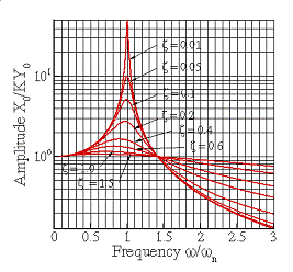
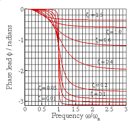
Solution for External Forcing
Equation of Motion
with
Steady State Solution:
The expressions for and
are graphed below, as a function of
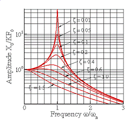

(a) (b)
Steady state vibration of a force spring-mass system (a) amplitude (b) phase.
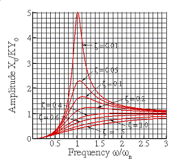
Solution for Base Excitation
Equation of Motion
with
Steady State solution
The expressions for and
are graphed below, as a function of
(a) (b)
Steady state
vibration of a base excited springmass
system (a) Amplitude and (b) phase
Solution for Rotor Excitation
Equation of Motion
with
Steady state solution
The expressions for and
are graphed below, as a function of
(a) (b)
Steady state
vibration of a rotor excited springmass
system (a) Amplitude (b) Phase
5.4.4 Features of the Steady State Response of Spring Mass Systems to Forced Vibrations.
Now, we will discuss the implications of the results in the preceding section.
![]() The
steady state response is always harmonic, and has the same frequency as that of
the forcing.
The
steady state response is always harmonic, and has the same frequency as that of
the forcing.
To see this mathematically, note that
in each case the solution has the form . Recall that
defines the frequency of the force, the
frequency of base excitation, or the rotor angular velocity. Thus, the frequency of vibration is
determined by the forcing, not by the properties of the spring-mass
system. This is unlike the free
vibration response.
You can also check this out using our
applet. To switch off the transient
solution, click on the checkbox labeled `show transient’. Then, try running the applet with different
values for k, m and ,
as well as different forcing frequencies, to see what happens. As long as you have switched off the
transient solution, the response will always be harmonic.
![]() The amplitude of vibration is
strongly dependent on the frequency of excitation, and on the properties of the
spring
The amplitude of vibration is
strongly dependent on the frequency of excitation, and on the properties of the
springmass
system.
To see this mathematically, note that
the solution has the form . Observe that
is the amplitude of vibration, and look at the
preceding section to find out how the amplitude of vibration varies with
frequency, the natural frequency of the system, the damping factor, and the
amplitude of the forcing. The formulae
for
are quite complicated, but you will learn a
great deal if you are able to sketch graphs of
as a function of
for various values of
.
You can also use our applet to study the influence of forcing frequency, the
natural frequency of the system, and the
damping coefficient. If you plot
position-v-time curves, make sure you switch off the transient solution to show
clearly the steady state behavior. Note
also that if you click on the `amplitude v-
frequency’ radio button just below the graphs, you will see a graph showing the
steady state amplitude of vibration as a function of forcing frequency. The current frequency of excitation is marked
as a square dot on the curve (if you don’t see the square dot, it means the
frequency of excitation is too high to fit on the scale
if you lower the excitation frequency and
press `start’ again you should see the dot appear). You can change the properties of the spring
mass system (or the natural frequency and damping coefficient) and draw new
amplitude-v-frequency curves to see how the response of the system has
changed.
Try the following tests
(i) Keeping the natural frequency fixed (or k and m fixed), plot ampltude-v-frequency graphs for various values of damping coefficient (or the dashpot coefficient). What happens to the maximum amplitude of vibration as damping is reduced?
(ii) Keep the damping coefficient fixed at around 0.1. Plot graphs of amplitude-v-frequency for various values of the natural frequency of the system. How does the maximum vibration amplitude change as natural frequency is varied? What about the frequency at which the maximum occurs?
(iii) Keep the dashpot coefficient fixed at a lowish value. Plot graphs of amplitude-v-frequency for various values of spring stiffness and mass. Can you reconcile the behavior you observe with the results of test (ii)?
(iv) Try changing the type of forcing to base excitation and rotor excitation. Can you see any differences in the amplitude-v-frequency curves for different types of forcing?
(v) Set the damping coefficient to a low value (below 0.1). Keep the natural frequency fixed. Run the program for different excitation frequencies. Watch what the system is doing. Observe the behavior when the excitation frequency coincides with the natural frequency of the system. Try this test for each type of excitation.
![]() If the forcing
frequency is close to the natural frequency of the system, and the system is
lightly damped, huge vibration amplitudes may occur. This phenomenon is known as resonance.
If the forcing
frequency is close to the natural frequency of the system, and the system is
lightly damped, huge vibration amplitudes may occur. This phenomenon is known as resonance.
If you ran the tests in the preceding section, you will have seen the system resonate. Note that the system resonates at a very similar frequency for each type of forcing.
As a general rule, engineers try to avoid resonance like the plague. Resonance is bad vibrations, man. Large amplitude vibrations imply large forces; and large forces cause material failure. There are exceptions to this rule, of course. Musical instruments, for example, are supposed to resonate, so as to amplify sound. Musicians who play string, wind and brass instruments spend years training their lips or bowing arm to excite just the right vibration modes in their instruments to make them sound perfect.
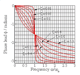
![]() There is a phase lag between the
forcing and the system response, which depends on the frequency of excitation
and the properties of the spring-mass system.
There is a phase lag between the
forcing and the system response, which depends on the frequency of excitation
and the properties of the spring-mass system.
The response of the system is . Expressions for
are given in the preceding section. Note that the phase lag is always
negative.
You can use the applet to examine the physical significance of the phase lag. Note that you can have the program plot a graph of phase-v-frequency for you, if you wish.
It is rather unusual to be particularly interested in the phase of the vibration, so we will not discuss it in detail here.
5.4.5 Engineering implications of vibration behavior
The solutions listed in the preceding sections give us
general guidelines for engineering a system to avoid (or create!) vibrations.
Preventing a system from vibrating: Suppose that we need to stop a structure or component
from vibrating e.g. to stop a tall building from
swaying. Structures are always
deformable to some extent
this is represented qualitatively by the
spring in a spring-mass system. They
always have mass
this is represented by the mass of the
block. Finally, the damper represents
energy dissipation. Forces acting on a
system generally fluctuate with time.
They probably aren’t perfectly harmonic, but they usually do have a fairly
well defined frequency (visualize waves on the ocean, for example, or wind
gusts. Many vibrations are man-made, in
which case their frequency is known
for example vehicles traveling on a road tend
to induce vibrations with a frequency of about 2Hz, corresponding to the bounce
of the car on its suspension).
So how do we stop the system from vibrating? We know that its motion is given by
To
minimize vibrations, we must design the system to make the vibration amplitude
Designing a suspension
or vibration isolation system. Suspensions, and vibration
isolation systems, are examples of base excited systems. In this case, the system really consists of a
mass (the vehicle, or the isolation table) on a spring (the shock absorber or
vibration isolation pad). We expect that
the base will vibrate with some characteristic frequency
Our vibration solution predicts that the mass vibrates
with displacement
Again,
the graph is helpful to understand how the vibration amplitude varies with system parameters.
Clearly,
we can minimize the vibration amplitude of the mass by making . We can do this by making the spring
stiffness as small as possible (use a soft spring), and making the mass
large. It also helps to make the damping
small.
This is counter-intuitive
people often think that the energy dissipated
by the shock absorbers in their suspensions that makes them work. There
are some disadvantages to making the damping too small, however. For one thing, if the system is lightly
damped, and is disturbed somehow, the subsequent transient vibrations will take
a very long time to die out. In
addition, there is always a risk that the frequency of base excitation is lower
than we expect
if the system is lightly damped, a potentially
damaging resonance may occur.
Suspension
design involves a bit more than simply minimizing the vibration of the mass, of
course the car will handle poorly if the wheels begin
to leave the ground. A very soft
suspension generally has poor handling, so the engineers must trade off
handling against vibration isolation.
5.4.6 Using Forced Vibration Response to Measure Properties of a System.
We often measure the natural frequency and damping coefficient for a mode of vibration in a structure or component, by measuring the forced vibration response of the system.
Here is how this is done. We find some way to apply a harmonic excitation to the system (base excitation might work; or you can apply a force using some kind of actuator, or you could deliberately mount an unbalanced rotor on the system).
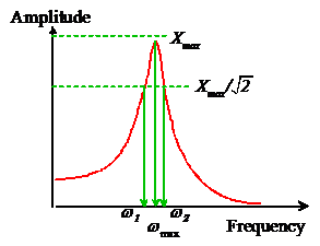
Then, we mount accelerometers on our system, and use them to measure the displacement of the structure, at the point where it is being excited, as a function of frequency.
We
then plot a graph, which usually looks something like the picture on the right.
We read off the maximum response ,
and draw a horizontal line at amplitude
. Finally, we measure the frequencies
,
and
as shown in the picture.
We define the bandwidth of the response as
Like the logarithmic decrement, the bandwidth of the forced harmonic response is a measure of the damping in a system.
It turns out that we can estimate the natural frequency of the system and its damping coefficient using the following formulae
The formulae are accurate
for small - say
.
To understand the origin of these formulae, recall that the amplitude of vibration due to external forcing is given by
We can find the frequency
at which the amplitude is a maximum by differentiating with respect to ,
setting the derivative equal to zero and solving the resulting equation for
frequency. It turns out that the maximum
amplitude occurs at a frequency
For small ,
we see that
Next, to get an expression
relating the bandwidth to
,
we first calculate the frequencies
and
. Note that the maximum amplitude of vibration
can be calculated by setting
,
which gives
Now, at the two frequencies
of interest, we know ,
so that
and
must be solutions of the equation
Rearrange this equation to see that
This is a quadratic
equation for and has solutions
Expand both expressions in
a Taylor series about to see that
so, finally, we confirm that
5.4.7 Example Problems in Forced Vibrations
Example 1: A
structure is idealized as a damped springmass
system with stiffness 10 kN/m; mass 2Mg; and dashpot coefficient 2 kNs/m. It is subjected to a harmonic force of
amplitude 500N at frequency 0.5Hz.
Calculate the steady state amplitude of vibration.
Start by calculating the properties of the system:
Now, the list of solutions to forced vibration problems gives
For the present problem:
Substituting numbers into the expression for the vibration amplitude shows that
Example 2: A
car and its suspension system are idealized as a damped springmass
system, with natural frequency 0.5Hz and damping coefficient 0.2. Suppose the car drives at speed V over a road with sinusoidal roughness. Assume the roughness wavelength is 10m, and
its amplitude is 20cm. At what speed
does the maximum amplitude of vibration occur, and what is the corresponding
vibration amplitude?
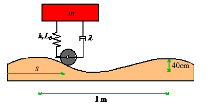
Let s denote the distance traveled by the car, and let L denote the wavelength of the roughness and H the roughness amplitude. Then, the height of the wheel above the mean road height may be expressed as
Noting that ,
we have that
i.e., the wheel oscillates
vertically with harmonic motion, at frequency .
Now, the suspension has
been idealized as a springmass
system subjected to base excitation. The
steady state vibration is
For light damping, the maximum amplitude of vibration occurs at around the natural frequency. Therefore, the critical speed follows from
Note that K=1 for base excitation, so that the
amplitude of vibration at is approximately
Note that at this speed, the suspension system is making the vibration worse. The amplitude of the car’s vibration is greater than the roughness of the road. Suspensions work best if they are excited at frequencies well above their resonant frequencies.
Example 3: The suspension system discussed in the preceding problem has the following specifications. For the roadway described in the preceding section, the amplitude of vibration may not exceed 35cm at any speed. At 55 miles per hour, the amplitude of vibration must be less than 10cm. The car weighs 3000lb. Select values for the spring stiffness and the dashpot coefficient.
We
must first determine values for and
that will satisfy the design specifications.
To this end:
(i)
The specification requires that
at resonance.
Examine the graph of shown with the solutions to the equations of
motion. Recall that K=1 for a base excited spring
mass
system. Observe that, with
,
the amplification factor never exceeds 1.75.
(ii) Now, the frequency of excitation at 55mph is
We must choose system parameters so that, at this
excitation frequency, .
Examine the graph showing the response of a base excited spring
mass
system again. We observe that, for
,
for
. Therefore, we pick
.
Finally, we can compute properties of the system. We have that
Similarly