5.2 Free vibration of conservative, single degree of freedom, linear systems.

 

First, we will explain what is meant by the title of this section.

       Recall that a system is conservative if energy is conserved, i.e. potential energy + kinetic energy = constant during motion.

       Free vibration means that no time varying external forces act on the system. 

       A system has one degree of freedom if its motion can be completely described by a single scalar variable.  We’ll discuss this in a bit more detail later.

        A system is said to be linear if its equation of motion is linear.  We will see what this means shortly.

 

It turns out that all 1DOF, linear conservative systems behave in exactly the same way.  By analyzing the motion of one representative system, we can learn about all others.

We will follow standard procedure, and use a spring-mass system as our representative example.

 

Problem:  The figure shows a spring mass system.  The spring has stiffness k and unstretched length .  The mass is released with velocity  from position  at time .  Find .

 

There is a standard approach to solving problems like this

 

(i) Get a differential equation for s using F=ma (or other methods to be discussed)

(ii) Solve the differential equation.

The picture shows a free body diagram for the mass.

 

 Newton’s law of motion states that

 

The spring force is related to the length of the spring by .  The i component of the equation of motion and this equation then shows that

 

This is our equation of motion for s.

 

Now, we need to solve this equation.  We could, of course, use Mathematica to do this  in fact here is the Mathematica solution.  

 

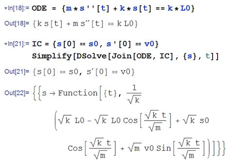
This is the correct solution  but Mathematica gives the result in a rather more complicated form than necessary.   For nearly all simple vibration problems, it is actually simpler just to write down the solution.  We will discuss the general procedure you should follow to do this in the next section.

 

5.2.1 How to solve equations of motion for vibration problems

 

Note that all vibrations problems have similar equations of motion.  Consequently, we can just solve the equation once, record the solution, and use it to solve any vibration problem we might be interested in.  The procedure to solve any vibration problem is:

1.      Derive the equation of motion, using Newton’s laws (or sometimes you can use energy methods, as discussed in Section 5.3)

2.      Do some algebra to arrange the equation of motion into a standard form

3.      Look up the solution to this standard form in a table of solutions to vibration problems.

 

We have provided a table of standard solutions as a separate document that you can download and print for future reference.

 

We will illustrate the procedure using many examples.

 

5.2.2 Solution to the equation of motion for an undamped spring-mass system

We would like to solve

 

with initial conditions   from position  at time .

 

We therefore consult our list of solutions to differential equations, and observe that it gives the solution to the following equation

 

 

This is very similar to our equation, but not identical.  To see how to get our equation into this form, note that (i) the standard equation has no coefficient in front of the x; and (ii) its right hand side is zero.  We can get our equation to look like this if we divide both sides by k, and subtract  from both sides of the equation.  This gives

 

Finally, we see that if we define

 

then our equation is equivalent to the standard one.

 

HEALTH WARNING: it is important to note that this substitution only works if  is constant, so its time derivative is zero.

 

The solution for x is

 

Here,  and  are the initial value of x and  its time derivative, which must be computed from the initial values of s and its time derivative

 

 

When we present the solution, we have a choice of writing down the solution for x, and giving formulas for the various terms in the solution (this is what is usually done):

 

Alternatively, we can express all the variables in the standard solution in terms of  s

 

But this solution looks very messy (more like the Mathematica solution).

 

Observe that:

       The mass oscillates harmonically, as discussed in the preceding section;

        The angular frequency of oscillation, , is a characteristic property of the system, and is independent of the initial position or velocity of the mass.  This is a very important observation, and we will expand upon it below.  The characteristic frequency is known as the natural frequency of the system.

         Increasing the stiffness of the spring increases the natural frequency of the system;

         Increasing the mass reduces the natural frequency of the system.

 

 

 

5.2.3 Natural Frequencies and Mode Shapes.

 

We saw that the spring mass system described in the preceding section likes to vibrate at a characteristic frequency, known as its natural frequency. This turns out to be a property of all stable mechanical systems. 

 

All stable, unforced, mechanical systems vibrate harmonically at certain discrete frequencies, known as natural frequencies of the system.

 

For the springmass system, we found only one natural frequency.  More complex systems have several natural frequencies.  For example, the system of two masses shown below has two natural frequencies, given by

 

 

 

A system with three masses would have three natural frequencies, and so on.

 

In general, a system with more than one natural frequency will not vibrate harmonically.

 

For example, suppose we start the two mass system vibrating, with initial conditions

 

The response may be shown (see sect 5.5 if you want to know how) to be

 

with

 

 

In general, the vibration response will look complicated, and is not harmonic. The animation above shows a typical example (if you are using the pdf version of these notes the animation will not work - you can download the matlab code that creates this animation here and run it for yourself)

 However, if we choose the special initial conditions:

 

then the response is simply

 

i.e., both masses vibrate harmonically, at the first natural frequency, as shown in the animation to the right.   (To repeat this in the MATLAB code, edit the file to set A1=0.3 and A2=0)

 

Similarly, if we choose

 

then

 

i.e., the system vibrates harmonically, at the second natural frequency. (To repeat this in the MATLAB code, edit the file to set A2=0.3 and A1 = 0)

 

The special initial displacements of a system that cause it to vibrate harmonically are called  `mode shapes’ for the system.

 

If a system has several natural frequencies, there is a corresponding mode of vibration for each natural frequency.

 

The natural frequencies are arguably the single most important property of any mechanical system.  This is because, as we shall see, the natural frequencies coincide (almost) with the system’s resonant frequencies.  That is to say, if you apply a time varying force to the system, and choose the frequency of the force to be equal to one of the natural frequencies, you will observe very large amplitude vibrations.

 

When designing a structure or component, you generally want to control its natural vibration frequencies very carefully.  For example, if you wish to stop a system from vibrating, you need to make sure that all its natural frequencies are much greater than the expected frequency of any forces that are likely to act on the structure.  If you are designing a vibration isolation platform, you generally want to make its natural frequency much lower than the vibration frequency of the floor that it will stand on.  Design codes usually specify allowable ranges for natural frequencies of structures and components.

 

Once a prototype has been built, it is usual to measure the natural frequencies and mode shapes for a system.  This is done by attaching a number of accelerometers to the system, and then hitting it with a hammer (this is usually a regular rubber tipped hammer, which might be instrumented to measure the impulse exerted by the hammer during the impact).  By trial and error, one can find a spot to hit the device so as to excite each mode of vibration independent of any other.  You can tell when you have found such a spot, because the whole system vibrates harmonically.  The natural frequency and mode shape of each vibration mode is then determined from the accelerometer readings.

 

Impulse hammer tests can even be used on big structures like bridges or buildings  but you need a big hammer.  In a recent test on a new cable stayed bridge in France, the bridge was excited by first attaching a barge to the center span with a high strength cable; then the cable was tightened to raise the barge part way out of the water; then, finally, the cable was released rapidly to set the bridge vibrating.

 

 

5.2.4 Calculating the number of degrees of freedom (and natural frequencies) of a system

 

When you analyze the behavior a system, it is helpful to know ahead of time how many vibration frequencies you will need to calculate.  There are various ways to do this.   Here are some rules that you can apply:

 

 

The number of degrees of freedom is equal to the number of independent coordinates required to describe the motion.  This is only helpful if you can see by inspection how to describe your system.  For the spring-mass system in the preceding section, we know that the mass can only move in one direction, and so specifying the length of the spring s will completely determine the motion of the system.  The system therefore has one degree of freedom, and one vibration frequency.   Section 5.6 provides several more examples where it is fairly obvious that the system has one degree of freedom.

 

 

For a 2D system, the number of degrees of freedom can be calculated from the equation

 

where:

 is the number of rigid bodies in the system

p is the number of particles in the system

 is the number of constraints (or, if you prefer, independent reaction forces) in the system.

 

To be able to apply this formula you need to know how many constraints appear in the problem.  Constraints are imposed by things like rigid links, or contacts with rigid walls, which force the system to move in a particular way.   The numbers of constraints associated with various types of 2D connections are listed in the table below.  Notice that the number of constraints is always equal to the number of reaction forces you need to draw on an FBD to represent the joint

 

 

 

 

For a 3D system, the number of degrees of freedom can be calculated from the equation

 

where the symbols have the same meaning as for a 2D system.   A table of various constraints for 3D problems is given below.

 

 

 

5.2.4 Calculating natural frequencies for 1DOF conservative systems

 

In light of the discussion in the preceding section, we clearly need some way to calculate natural frequencies for mechanical systems.  We do not have time in this course to discuss more than the very simplest mechanical systems.  We will therefore show you some tricks for calculating natural frequencies of 1DOF, conservative, systems. It is best to do this by means of examples.

 

Example 1: The spring-mass system revisited

 

Calculate the natural frequency of vibration for the system shown in the figure. Assume that the contact between the block and wedge is frictionless.  The spring has stiffness k and unstretched length  

 

 Our first objective is to get an equation of motion for s.  We could do this by drawing a FBD, writing down Newton’s law, and looking at its components.  However, for 1DOF systems it turns out that we can derive the EOM very quickly using the kinetic and potential energy of the system. 

 

The potential energy and kinetic energy can be written down as:

 

(The second term in V is the gravitational potential energy  it is negative because the height of the mass decreases with increasing s).  Now, note  that since our system is conservative

 

Differentiate our expressions for T and V (use the chain rule) to see that

 

Finally, we must turn this equation of motion into one of the standard solutions to vibration equations.

Our equation looks very similar to

 

Thus let

 

and substitute into the equation of motion:

 

By comparing this with our equation we see that the natural frequency of vibration is

 

 

 

Summary of procedure for calculating natural frequencies:

 

(1)  Describe the motion of the system, using a single scalar variable (In the example, we chose to describe motion using the distance s);

(2) Write down the potential energy V and kinetic energy T of the system in terms of the scalar variable;

(3) Use  to get an equation of motion for your scalar variable;

(4) Arrange the equation of motion in standard form;

(5) Read off the natural frequency by comparing your equation to the standard form.

 

 

Example 2: A nonlinear system.

 

We will illustrate the procedure with a second example, which will demonstrate another useful trick.

 

Find the natural frequency of vibration for a pendulum, shown in the figure.

We will idealize the mass as a particle, to keep things simple.

 

We will follow the steps outlined earlier:

  (1)  We describe the motion using the angle  

  (2)  We write down T and V:

 

(if you don’t see the formula for the kinetic energy, you can write down the position vector of the mass as , differentiate to find the velocity: , and then compute  and use a trig identity.  You can also use the circular motion formulas, if you prefer).

 (3) Differentiate with respect to time:

 

 (4) Arrange the EOM into standard form.  Houston, we have a problem.  There is no way this equation can be arranged into standard form.  This is because the equation is nonlinear (  is a nonlinear function of  ).  There is, however, a way to deal with this problem.  We will show what needs to be done, summarizing the general steps as we go along.

 

 

(i) Find the static equilibrium configuration(s) for the system.

 

 If the system is in static equilibrium, it does not move.  We can find values of  for which the system is in static equilibrium by setting all time derivatives of  in the equation of motion to zero, and then solving the equation.  Here,

 

Here, we have used  to denote the special values of  for which the system happens to be in static equilibrium.  Note that  is always a constant.

 

(ii) Assume that the system vibrates with small amplitude about a static equilibrium configuration of interest.

 

To do this, we let , where .

 

Here, x represents a small change in angle from an equilibrium configuration.. Note that x will vary with time as the system vibrates.  Instead of solving for , we will solve for x.  Before going on, make sure that you are comfortable with the physical significance of  both x and .

 

(iii) Linearize the equation of motion, by expanding all nonlinear terms as Taylor Maclaurin series about the equilibrium configuration.

 

We substitute for  in the equation of motion, to see that

 

 

(Recall that  is constant, so its time derivatives vanish)

 

Now, recall the Taylor-Maclaurin series expansion of a function f(x) has the form

 

where

 

Apply this to the nonlinear term in our equation of motion

 

Now, since x<<1, we can assume that , and so

 

Finally, we can substitute back into our equation of motion, to obtain

 

 

(iv) Compare the linear equation with the standard form to deduce the natural frequency.

 

We can do this for each equilibrium configuration.

 

whence

 

Note that all these values of  really represent the same configuration: the mass is hanging below the pivot.  We have rediscovered the well-known expression for the natural frequency of a freely swinging pendulum.

 

Next, try the remaining static equilibrium configuration

 

If we look up this equation in our list of standard solutions, we find it does not have a harmonic solution.  Instead, the solution is

 

where  and  

 

Thus, except for some rather special initial conditions, x increases without bound as time increases.  This is a characteristic of an unstable mechanical system.

 

If we visualize the system with , we can see what is happening.  This equilibrium configuration has the pendulum upside down!

 

No wonder the equation is predicting an instability…

 

Here is a question to think about.  Our solution predicts that both x and dx/dt become infinitely large.  We know that a real pendulum would never rotate with infinite angular velocity.  What has gone wrong?

 

 

 

 

Example 3: We will look at one more nonlinear system, to make sure that you are comfortable with this procedure. Calculate the resonant frequency of small oscillations about the equilibrium configuration  for the system shown. The spring has stiffness k and unstretched length .

 

We follow the same procedure as before.

 

The potential and kinetic energies of the system are

 

Hence

 

Once again, we have found a nonlinear equation of motion.  This time we know what to do.  We are told to find natural frequency of oscillation about , so we don’t need to solve for the equilibrium configurations this time.  We set , with  and substitute back into the equation of motion:

 

Now, expand all the nonlinear terms (it is OK to do them one at a time and then multiply everything out.  You can always throw away all powers of x greater than one as you do so)

 

If you prefer, you can use Mathematica to do the Taylor series expansion:

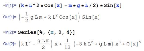
(The number 4 in the ‘series’ command specifies the highest power of x that should appear in the expansion). We now have an equation in standard form, and can read off the natural frequency

 

Question: what happens for ?

 

Example 3: A system with a rigid body (the KE of a rigid body will be defined in the next section of the course  just live with it for now!).

 

Calculate the natural frequency of vibration for the system shown in the figure.  Assume that the cylinder rolls without slip on the wedge. The spring has stiffness k and unstretched length  

 

Our first objective is to get an equation of motion for s.  We do this by writing down the potential and kinetic energies of the system in terms of s.

 

The potential energy is easy:

 

The first term represents the energy in the spring, while second term accounts for the gravitational potential energy.

 

The kinetic energy is slightly more tricky.  Note that the magnitude of the angular velocity of the disk is related to the magnitude of its translational velocity by

 

Thus, the combined rotational and translational kinetic energy follows as

 

 

Now, note that since our system is conservative

 

Differentiate our expressions for T and V to see that

 

The last equation is almost in one of the standard forms given on the handout, except that the right hand side is not zero.  There is a trick to dealing with this problem  simply subtract the constant right hand side from s, and call the result x.  (This only works if the right hand side is a constant, of course).  Thus let

 

and substitute into the equation of motion:

 

This is now in the form

 

and by comparing this with our equation we see that the natural frequency of vibration is