
5.5 Introduction to vibration of systems with many degrees of freedom
The
simple 1DOF systems analyzed in the preceding section are very helpful to
develop a feel for the general characteristics of vibrating systems. They are too simple to approximate most real
systems, however. Real systems have
more than just one degree of freedom.
Real systems are also very rarely linear. You may be feeling cheated are the simple idealizations that you get to
see in intro courses really any use? It
turns out that they are, but you can only really be convinced of this if you
know how to analyze more realistic problems, and see that they often behave
just like the simple idealizations.
The
motion of systems with many degrees of freedom, or nonlinear systems, cannot
usually be described using simple formulas. Even when they can, the formulas
are so long and complicated that you need a computer to evaluate them. For this reason, introductory courses
typically avoid these topics. However, if
you are willing to use a computer, analyzing the motion of these complex
systems is actually quite straightforward in fact, often easier than using the nasty
formulas we derived for 1DOF systems.
This section of the notes is intended mostly for advanced students, who may be insulted by simplified models. If you are feeling insulted, read on…
5.5.1 Equations of motion for undamped linear systems with many degrees of freedom.

We
always express the equations of motion for a system with many degrees of
freedom in a standard form. The two degree
of freedom system shown in the picture can be used as an example. We won’t go through the calculation in detail
here (you should be able to derive it for yourself draw a FBD, use Newton’s law and all that
tedious stuff), but here is the final answer:
To solve vibration problems, we always write the equations of motion in matrix form. For an undamped system, the matrix equation of motion always looks like this
where x is a vector of the variables describing the motion, M is called the ‘mass matrix’ and K is called the ‘Stiffness matrix’ for the system. For the two spring-mass example, the equation of motion can be written in matrix form as
For a system with two masses (or more generally, two degrees of freedom), M and K are 2x2 matrices. For a system with n degrees of freedom, they are nxn matrices.
 The spring-mass system is linear. A nonlinear system has more complicated
equations of motion, but these can always be arranged into the standard matrix
form by assuming that the displacement of the system is small, and linearizing
the equation of motion. For example, the
full nonlinear equations of motion for the double pendulum shown in the figure
are
The spring-mass system is linear. A nonlinear system has more complicated
equations of motion, but these can always be arranged into the standard matrix
form by assuming that the displacement of the system is small, and linearizing
the equation of motion. For example, the
full nonlinear equations of motion for the double pendulum shown in the figure
are
Here,
a single dot over a variable represents a time derivative, and a double dot
represents a second time derivative (i.e. acceleration). These equations look
horrible (and indeed they are the motion of a double pendulum can even be
chaotic), but if we assume that if
,
,
and their time derivatives are all small, so that terms involving squares, or
products, of these variables can all be neglected, that and recall that
and
for small x,
the equations simplify to
Or, in matrix form
This is again in the standard form.
Throughout the rest of this section, we will focus on exploring the behavior of systems of springs and masses. This is not because spring/mass systems are of any particular interest, but because they are easy to visualize, and, more importantly the equations of motion for a spring-mass system are identical to those of any linear system. This could include a realistic mechanical system, an electrical system, or anything that catches your fancy. (Then again, your fancy may tend more towards nonlinear systems, but if so, you should keep that to yourself).
5.5.2 Natural frequencies and mode shapes for undamped linear systems with many degrees of freedom.
First, let’s review the definition of natural frequencies and mode shapes. Recall that we can set a system vibrating by displacing it slightly from its static equilibrium position, and then releasing it. In general, the resulting motion will not be harmonic. However, there are certain special initial displacements that will cause harmonic vibrations. These special initial deflections are called mode shapes, and the corresponding frequencies of vibration are called natural frequencies.
The natural frequencies of a vibrating system are its most important property. It is helpful to have a simple way to calculate them.
Fortunately, calculating natural frequencies turns out to be quite easy (at least on a computer). Recall that the general form of the equation of motion for a vibrating system is
where x is a time dependent vector that describes the motion, and M and K are mass and stiffness matrices. Since we are interested in
finding harmonic solutions for x, we
can simply assume that the solution has the form ,
and substitute into the equation of motion
The
vectors u and scalars that satisfy a matrix equation of the form
are called ‘generalized eigenvectors’ and
‘generalized eigenvalues’ of the equation.
It is impossible to find exact formulas for
and u
for a large matrix (formulas exist for up to 5x5 matrices, but they are so
messy they are useless), but MATLAB has built-in functions that will compute
generalized eigenvectors and eigenvalues given numerical values for M and K.
The
special values of satisfying
are related to the natural frequencies by
The special vectors X are the ‘Mode shapes’ of the system. These are the special initial displacements that will cause the mass to vibrate harmonically.
If you only want to know the natural frequencies (common) you can use the MATLAB command
d = eig(K,M)
This
returns a vector d, containing all the values of satisfying
(for an nxn matrix, there are usually n different values). The natural frequencies follow as
.
If you want to find both the eigenvalues and eigenvectors, you must use
[V,D] = eig(K,M)
This returns two matrices, V and D. Each column of the
matrix V corresponds to a vector u that
satisfies the equation, and the diagonal elements of D contain the
corresponding value of . To extract the ith frequency and mode shape,
use
omega = sqrt(D(i,i))
X = V(:,i)
For example, here is a MATLAB function that uses this function to automatically compute the natural frequencies of the spring-mass system shown in the figure.
function [freqs,modes] = compute_frequencies(k1,k2,k3,m1,m2)
M = [m1,0;0,m2];
K = [k1+k2,-k2;-k2,k2+k3];
[V,D] = eig(K,M);
for i = 1:2
freqs(i) = sqrt(D(i,i));
end
modes = V;
end
You could try running this with
>> [freqs,modes] = compute_frequencies(2,1,1,1,1)
This
gives the natural frequencies as ,
and the mode shapes as
(i.e. both masses displace in the same
direction) and
(the two masses displace in opposite
directions.
If
you read textbooks on vibrations, you will find that they may give different
formulas for the natural frequencies and vibration modes. (If you read a lot of
textbooks on vibrations there is probably something seriously wrong with your
social life). This is partly because
solving for
and u
is rather complicated (especially if you have to do the calculation by hand), and
partly because this formula hides some subtle mathematical features of the
equations of motion for vibrating systems.
For example, the solutions to
are generally complex (
and u
have real and imaginary parts), so it is not obvious that our guess
actually satisfies the equation of
motion. It turns out, however, that the equations
of motion for a vibrating system can always be arranged so that M and K are symmetric. In this
case
and u are
real, and
is always positive or zero. The old fashioned formulas for natural frequencies
and vibration modes show this more clearly.
But our approach gives the same answer, and can also be generalized
rather easily to solve damped systems (see Section 5.5.5), whereas the
traditional textbook methods cannot.
5.5.3 Free vibration of undamped linear systems with many degrees of freedom.
As
an example, consider a system with n
identical masses with mass m, connected
by springs with stiffness k, as shown
in the picture. Suppose that at time t=0 the masses are displaced from their
static equilibrium position by distances ,
and have initial speeds
. We would like to calculate the motion of each
mass
as a function of time.
It is convenient to represent the initial displacement and velocity as n dimensional vectors u and v, as
,
and
. In addition, we must calculate the natural
frequencies
and mode shapes
,
i=1..n for the system. The motion can then be calculated using the
following formula
where
Here, the dot represents an n dimensional dot product (to evaluate it in matlab, just use the dot() command).
This
expression tells us that the general vibration of the system consists of a sum
of all the vibration modes, (which all vibrate at their own discrete
frequencies). You can control how big
the contribution is from each mode by starting the system with different
initial conditions. The mode shapes have the curious property that the dot
product of two different mode shapes is always zero (
,
etc)
so you can see that if the initial displacements
u happen to be the same as a mode
shape, the vibration will be harmonic.
The figure on the right animates the motion of a system with 6 masses, which is set in motion by displacing the leftmost mass and releasing it. The graph shows the displacement of the leftmost mass as a function of time. You can download the MATLAB code for this computation here, and see how the formulas listed in this section are used to compute the motion. The program will predict the motion of a system with an arbitrary number of masses, and since you can easily edit the code to type in a different mass and stiffness matrix, it effectively solves any transient vibration problem.
5.5.4 Forced vibration of lightly damped linear systems with many degrees of freedom.
It is quite simple to find a formula for the motion of an undamped system subjected to time varying forces. The predictions are a bit unsatisfactory, however, because their vibration of an undamped system always depends on the initial conditions. In a real system, damping makes the steady-state response independent of the initial conditions. However, we can get an approximate solution for lightly damped systems by finding the solution for an undamped system, and then neglecting the part of the solution that depends on initial conditions.
As
an example, we will consider the system with two springs and masses shown in
the picture. Each mass is subjected to a
harmonic force, which vibrates with some frequency (the forces acting on the different masses all
vibrate at the same frequency). The equations of motion are
We can write these in matrix form as
or, more generally,
To
find the steady-state solution, we simply assume that the masses will all
vibrate harmonically at the same frequency as the forces. This means that ,
,
where
are the (unknown) amplitudes of vibration of
the two masses. In vector form we could
write
,
where
. Substituting this into the equation of motion
gives
This is a system of linear equations for X. They can easily be solved using MATLAB. As an example, here is a simple MATLAB function that will calculate the vibration amplitude for a linear system with many degrees of freedom, given the stiffness and mass matrices, and the vector of forces f.
function X = forced_vibration(K,M,f,omega)
% Function to calculate steady state amplitude of
% a forced linear system.
% K is nxn the stiffness matrix
% M is the nxn mass matrix
% f is the n dimensional force vector
% omega is the forcing frequency, in radians/sec.
% The function computes a vector X, giving the amplitude of
% each degree of freedom
%
X = (K-M*omega^2)\f;
end
The function is only one line long!
As
an example, the graph below shows the predicted steady-state vibration
amplitude for the spring-mass system, for the special case where the masses are
all equal ,
and the springs all have the same stiffness
. The first mass is subjected to a harmonic
force
,
and no force acts on the second mass. Note
that the graph shows the magnitude of the vibration amplitude
the formula predicts that for some frequencies
some masses have negative vibration amplitudes, but the negative sign has been
ignored, as the negative sign just means that the mass vibrates out of phase
with the force.
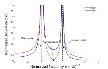
Several features of the result are worth noting:
![]() If the forcing frequency is close to
any one of the natural frequencies of the system, huge vibration amplitudes
occur. This phenomenon is known as resonance. You can check the natural frequencies of the
system using the little matlab code in section 5.5.2
If the forcing frequency is close to
any one of the natural frequencies of the system, huge vibration amplitudes
occur. This phenomenon is known as resonance. You can check the natural frequencies of the
system using the little matlab code in section 5.5.2 they turn out to be
and
. At these frequencies the vibration amplitude
is theoretically infinite.
![]()
 The figure predicts an intriguing new
phenomenon
The figure predicts an intriguing new
phenomenon at a magic frequency, the amplitude of
vibration of mass 1 (that’s the mass that the force acts on) drops to
zero. This is called ‘Anti-resonance,’
and it has an important engineering application. Suppose that we have designed a system with a
serious vibration problem (like the London Millenium bridge). Usually, this occurs because some kind of
unexpected force is exciting one of the vibration modes in the system. We can idealize this behavior as a
mass-spring system subjected to a force, as shown in the figure. So how do we stop the system from
vibrating? Our solution for a 2DOF
system shows that a system with two masses will have an anti-resonance. So we simply turn our 1DOF system into a 2DOF
system by adding another spring and a mass, and tune the stiffness and mass of
the new elements so that the anti-resonance occurs at the appropriate frequency. Of course, adding a mass will create a new
vibration mode, but we can make sure that the new natural frequency is not at a
bad frequency. We can also add a
dashpot in parallel with the spring, if we want
this has the effect of making the
anti-resonance phenomenon somewhat less effective (the vibration amplitude will
be small, but finite, at the ‘magic’ frequency), but the new vibration modes
will also have lower amplitudes at resonance. The added spring
mass system is called a ‘tuned vibration
absorber.’ This approach was used to solve the Millenium Bridge
vibration problem.
5.5.5 The effects of damping
 In most design calculations, we don’t worry about
accounting for the effects of damping very accurately. This is partly because it’s very difficult to
find formulas that model damping realistically, and even more difficult to find
values for the damping parameters.
Also, the mathematics required to solve damped problems is a bit messy.
Old textbooks don’t cover it, because for practical purposes it is only
possible to do the calculations using a computer. It is not hard to account for the effects of
damping, however, and it is helpful to have a sense of what its effect will be
in a real system. We’ll go through this
rather briefly in this section.
In most design calculations, we don’t worry about
accounting for the effects of damping very accurately. This is partly because it’s very difficult to
find formulas that model damping realistically, and even more difficult to find
values for the damping parameters.
Also, the mathematics required to solve damped problems is a bit messy.
Old textbooks don’t cover it, because for practical purposes it is only
possible to do the calculations using a computer. It is not hard to account for the effects of
damping, however, and it is helpful to have a sense of what its effect will be
in a real system. We’ll go through this
rather briefly in this section.
Equations of motion: The figure shows a damped spring-mass system. The equations of motion for the system can easily be shown to be
To
solve these equations, we have to reduce them to a system that MATLAB can
handle, by re-writing them as first order equations. We follow the standard procedure to do this define
and
as new variables, and then write the equations
in matrix form as
(This result might not be
obvious to you if so, multiply out the vector-matrix products
to see that the equations are all correct). This is a matrix equation of the
form
where y is a vector containing the unknown velocities and positions of the mass.
Free vibration response: Suppose that at time t=0 the system has initial positions and velocities ,
and we wish to calculate the subsequent motion of the system. To do this, we
must solve the equation of motion. We start by guessing that the solution has
the form
(the negative sign is introduced because we
expect solutions to decay with time).
Here,
is a constant vector, to be determined. Substituting this into the equation of
motion gives
This
is another generalized eigenvalue problem, and can easily be solved with
MATLAB. The solution is much more
complicated for a damped system, however, because the possible values of and
that satisfy the equation are in general complex
that is to say, each
can be expressed as
,
where
and
are positive real numbers, and
. This makes more sense if we recall Euler’s
formula
(if
you haven’t seen Euler’s formula, try doing a Taylor expansion of both sides of
the equation you will find they are magically equal. If you don’t know how to do a Taylor
expansion, you probably stopped reading this ages ago, but if you are still
hanging in there, just trust me…). So,
the solution is predicting that the response may be oscillatory, as we would
expect. Once all the possible vectors
and
have been calculated, the response of the
system can be calculated as follows:
1.
Construct a
matrix H , in which each column is
one of the possible values of (MATLAB constructs this matrix automatically)
2. Construct a diagonal matrix (t), which has the form
where
each is one of the solutions to the generalized
eigenvalue equation.
3. Calculate a vector a (this represents the amplitudes of the various modes in the vibration response) that satisfies
4. The vibration response then follows as
All
the matrices and vectors in these formulas are complex valued but all the imaginary parts magically
disappear in the final answer.
HEALTH WARNING: The formulas listed here only work if all the generalized
eigenvalues satisfying
are different. For some very special choices of damping,
some eigenvalues may be repeated. In
this case the formula won’t work. A
quick and dirty fix for this is just to change the damping very slightly, and
the problem disappears. Your applied
math courses will hopefully show you a better fix, but we won’t worry about
that here.
 This all sounds a bit involved, but it actually only
takes a few lines of MATLAB code to calculate the motion of any damped system.
As an example, a MATLAB code that animates the motion of a damped spring-mass
system shown in the figure (but with an arbitrary number of masses) can be
downloaded here. You can use the code
to explore the behavior of the system.
In addition, you can modify the code to solve any linear free vibration
problem by modifying the matrices M
and D.
This all sounds a bit involved, but it actually only
takes a few lines of MATLAB code to calculate the motion of any damped system.
As an example, a MATLAB code that animates the motion of a damped spring-mass
system shown in the figure (but with an arbitrary number of masses) can be
downloaded here. You can use the code
to explore the behavior of the system.
In addition, you can modify the code to solve any linear free vibration
problem by modifying the matrices M
and D.
Here
are some animations that illustrate the behavior of the system. The animations
below show vibrations of the system with initial displacements corresponding to
the three mode shapes of the undamped system (calculated using the procedure in
Section 5.5.2). The results are shown
for k=m=1 .
In each case, the graph plots the motion of the three masses
if a color doesn’t show up, it means one of
the other masses has the exact same displacement.
Mode 1 Mode 2 Mode 3
Notice that
1. For each mode, the displacement history of any mass looks very similar to the behavior of a damped, 1DOF system.
2. The amplitude of the high frequency modes die out much faster than the low frequency mode.
 This explains why it is so helpful to understand the
behavior of a 1DOF system. If a more
complicated system is set in motion, its response initially involves
contributions from all its vibration modes.
Soon, however, the high frequency modes die out, and the dominant
behavior is just caused by the lowest frequency mode. The animation to the
right demonstrates this very nicely
This explains why it is so helpful to understand the
behavior of a 1DOF system. If a more
complicated system is set in motion, its response initially involves
contributions from all its vibration modes.
Soon, however, the high frequency modes die out, and the dominant
behavior is just caused by the lowest frequency mode. The animation to the
right demonstrates this very nicely here, the system was started by displacing
only the first mass. The initial
response is not harmonic, but after a short time the high frequency modes stop
contributing, and the system behaves just like a 1DOF approximation. For design purposes, idealizing the system as
a 1DOF damped spring-mass system is usually sufficient.
Notice
also that light damping has very little effect on the natural frequencies and
mode shapes so the simple undamped approximation is a good
way to calculate these.
Of
course, if the system is very heavily damped, then its behavior changes
completely the system no longer vibrates, and instead
just moves gradually towards its equilibrium position. You can simulate this behavior for yourself
using the matlab code
try running it with
or higher.
Systems of this kind are not of much practical interest.
Steady-state forced vibration response. Finally, we take a look at the effects of damping on the response of a spring-mass system to harmonic forces. The equations of motion for a damped, forced system are
This is an equation of the form
where we have used Euler’s famous formula again. We can find a solution to
by guessing that ,
and substituting into the matrix equation
This equation can be solved
for . Similarly, we can solve
by
guessing that ,
which gives an equation for
of the form
.
You actually don’t need to solve this equation
you can simply calculate
by just changing the sign of all the imaginary
parts of
.
The full solution follows as
This is the steady-state vibration response. Just as for the 1DOF system, the general solution also has a transient part, which depends on initial conditions. We know that the transient solution will die away, so we ignore it.
The
solution for y(t) looks peculiar,
because of the complex numbers. If we
just want to plot the solution as a function of time, we don’t have to worry
about the complex numbers, because they magically disappear in the final
answer. In fact, if we use MATLAB to do
the computations, we never even notice that the intermediate formulas involve
complex numbers. If we do plot the solution,
it is obvious that each mass vibrates harmonically, at the same frequency as
the force (this is obvious from the formula too). It’s not worth plotting the function we are really only interested in the amplitude
of vibration of each mass. This can be calculated as follows
1.
Let ,
denote the components of
and
2. The vibration of the jth mass then has the form
where
are the amplitude and phase of the harmonic vibration of the mass.
If
you know a lot about complex numbers you could try to derive these formulas for
yourself. If not, just trust me your math classes should cover this kind of
thing. MATLAB can handle all these
computations effortlessly. As an
example, here is a simple MATLAB script that will calculate the steady-state
amplitude of vibration and phase of each degree of freedom of a forced n degree of freedom system, given the
force vector f, and the matrices M and D that describe the system.
function [amp,phase] = damped_forced_vibration(D,M,f,omega)
% Function to calculate steady state amplitude of
% a forced linear system.
% D is 2nx2n the stiffness/damping matrix
% M is the 2nx2n mass matrix
% f is the 2n dimensional force vector
% omega is the forcing frequency, in radians/sec.
% The function computes a vector ‘amp’, giving the amplitude of
% each degree of freedom, and a second vector ‘phase’,
% which gives the phase of each degree of freedom
%
Y0 = (D+M*i*omega)\f; % The i here is sqrt(-1)
% We dont need to calculate Y0bar - we can just change the sign of
% the imaginary part of Y0 using the 'conj' command
for j =1:length(f)/2
amp(j) = sqrt(Y0(j)*conj(Y0(j)));
phase(j) = log(conj(Y0(j))/Y0(j))/(2*i);
end
end
Again, the script is very simple.
Here is a graph showing the predicted vibration amplitude of each mass in the system shown. Note that only mass 1 is subjected to a force.
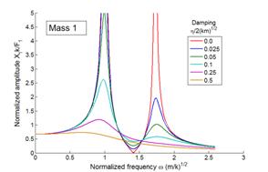
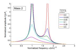
The important conclusions to be drawn from these results are:
1. We observe two resonances, at frequencies very close to the undamped natural frequencies of the system.
2. For light damping, the undamped model predicts the vibration amplitude quite accurately, except very close to the resonance itself (where the undamped model has an infinite vibration amplitude)
3.
In a damped
system, the amplitude of the lowest frequency resonance is generally much
greater than higher frequency modes. For
this reason, it is often sufficient to consider only the lowest frequency mode in
design calculations. This means we can
idealize the system as just a single DOF system, and think of it as a simple
spring-mass system as described in the early part of this chapter. The relative vibration amplitudes of the
various resonances do depend to some extent on the nature of the force it is possible to choose a set of forces that
will excite only a high frequency
mode, in which case the amplitude of this special excited mode will exceed all
the others. But for most forcing, the
lowest frequency one is the one that matters.
4. The ‘anti-resonance’ behavior shown by the forced mass disappears if the damping is too high.