EN4: Dynamics and Vibrations

 

Division of Engineering
Brown University

 

6.7 Free vibration of a damped, single degree of freedom, linear spring mass system.

We analyzed vibration of several conservative systems in the preceding section. In each case, we found that if the system was set in motion, it continued to move indefinitely. This is counter to our everyday experience. Usually, if you start something vibrating, it will vibrate with a progressively decreasing amplitude and eventually stop moving.

The reason our simple models predict the wrong behavior is that we neglected energy dissipation. In this section, we explore the influence of energy dissipation on free vibration of a spring-mass system. As before, although we model a very simple system, the behavior we predict turns out to be representative of a wide range of real engineering systems.

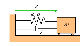
Problem: The spring mass dashpot system shown is released with velocity from position at time . Find .

Once again, we follow the standard approach to solving problems like this

(i) Get a differential equation for s using F=ma

(ii) Solve the differential equation.

You may have forgotten what a dashpot (or damper) does. Suppose we apply a force F to a dashpot, as shown below:

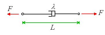
We would observe that the dashpot stretched at a rate proportional to the force

One can buy dampers (the shock absorbers in your car contain dampers): a damper generally consists of a plunger inside an oil filled cylinder, which dissipates energy by churning the oil. Thus, it is possible to make a spring-mass-damper system that looks very much like the one in the picture. More generally, however, the spring mass system is used to represent a complex mechanical system. In this case, the damper represents the combined effects of all the various mechanisms for dissipating energy in the system, including friction, air resistance, deformation losses, and so on.

To proceed, we draw a free body diagram, showing the forces exerted by the spring and damper on the mass.

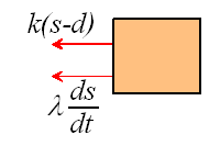
Newton II states that

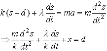
This is our equation of motion for s.

Now, we check our list of solutions to differential equations, and see that we have a solution to:

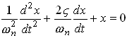
We can get our equation into this form by setting

 

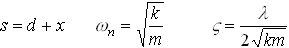
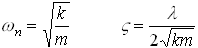
As before, is known as the natural frequency of the system. We have discovered a new parameter, , which is called the damping coefficient. It plays a very important role, as we shall see below.

 

Now, we can write down the solution for x:

Overdamped System

where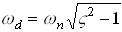

Critically Damped System

Underdamped System

where is known as the damped natural frequency of the system.

In all the preceding equations,

are the values of x and its time derivative at time t=0.

These expressions are rather too complicated to visualize what the system is doing for any given set of parameters. The applet below might help. You can use the sliders to set the values of either m, k, and (in this case the program will calculate the values of and for you, and display the results), or alternatively, you can set the values of and directly. You can also choose values for the initial conditions and . When you press `start’ the animation will show you the behavior of the system, and a graph of the position of the mass as a function of time will be drawn. You can also choose to display the phase plane, which shows the velocity of the mass as a function of its position, if you wish. You can stop the animation at any time, change the parameters, and plot a new graph on top of the first to see what has changed. If you press `reset’, all your graphs will be cleared, and you can start again.

 

 

 

Try the following tests to familiarize yourself with the behavior of the system

 Set the dashpot coefficient to a low value, so that the damping coefficient . Make sure the graph is set to display position versus time, and press `start.’ You should see the system vibrate. The vibration looks very similar to the behavior of the conservative system we analyzed in the preceding section, except that the amplitude decays with time. Note that the system vibrates at a frequency very slightly lower than the natural frequency of the system.

 Keeping the value of fixed, vary the values of spring constant and mass to see what happens to the frequency of vibration and also to the rate of decay of vibration. Is the behavior consistent with the solutions given above?

 Keep the values of k and m fixed, and vary . You should see that, as you increase , the vibration dies away more and more quickly. What happens to the frequency of oscillations as is increased? Is this behavior consistent with the predictions of the theory?

 Now, set the damping coefficient (not the dashpot coefficient this time) to . For this value, the system no longer vibrates; instead, the mass smoothly returns to its equilibrium position x=0. If you need to design a system that returns to its equilibrium position in the shortest possible time, then it is customary to select system parameters so that . A system of this kind is said to be critically damped.

 Set to a value greater than 1. Under these conditions, the system decays more slowly towards its equilibrium configuration.

 Keeping >1, experiment with the effects of changing the stiffness of the spring and the value of the mass. Can you explain what is happening mathematically, using the equations of motion and their solution?

 Finally, you might like to look at the behavior of the system on its phase plane. In this course, we will not make much use of the phase plane, but it is a powerful tool for visualizing the behavior of nonlinear systems. By looking at the patterns traced by the system on the phase plane, you can often work out what it is doing. For example, if the trajectory encircles the origin, then the system is vibrating. If the trajectory approaches the origin, the system is decaying to its equilibrium configuration.

 

We now know the effects of energy dissipation on a vibrating system. One important conclusion is that if the energy dissipation is low, the system will vibrate. Furthermore, the frequency of vibration is very close to that of an undamped system. Consequently, if you want to predict the frequency of vibration of a system, you can simplify the calculation by neglecting damping.

 

6.8 Using Free Vibrations to Measure Properties of a System

We will describe one very important application of the results developed in the preceding section.

It often happens that we need to measure the dynamical properties of an engineering system. For example, we might want to measure the natural frequency and damping coefficient for a structure after it has been built, to make sure that design predictions were correct, and to use in future models of the system.

You can use the free vibration response to do this, as follows.

First, you instrument your design by attaching accelerometers to appropriate points. You then use an impulse hammer to excite a particular mode of vibration, as discussed in Section 6.5. You use your accelerometer readings to determine the displacement at the point where the structure was excited: the results will be a graph similar to the one shown below.

 

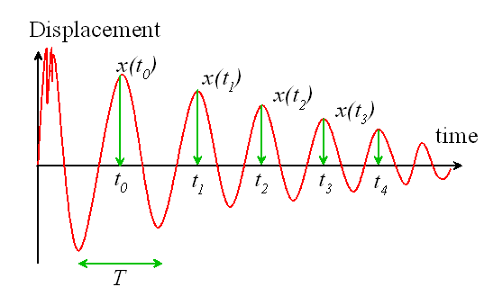
We then identify a nice looking peak, and call the time there , as shown.

The following quantities are then measured from the graph:

1. The period of oscillation. The period of oscillation was defined in Section 6.2: it is the time between two peaks, as shown. Since the signal is (supposedly) periodic, it is often best to estimate T as follows

where is the time at which the nth peak occurs, as shown in the picture.

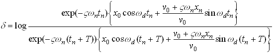
2. The Logarithmic Decrement. This is a new quantity, defined as follows

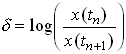
where is the displacement at the nth peak, as shown. In principle, you should be able to pick any two neighboring peaks, and calculate . You should get the same answer, whichever peaks you choose. It is often more accurate to estimate using the following formula

This expression should give the same answer as the earlier definition.

 

Now, it turns out that we can deduce and from T and , as follows.

 

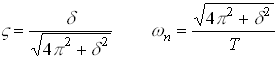
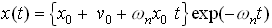
Why does this work? Let us calculate T and using the exact solution to the equation of motion for a damped spring-mass system. Recall that, for an underdamped system, the solution has the form

where

Hence, the period of oscillation is

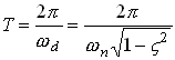
Similarly,

where we have noted that .

Fortunately, this horrendous equation can be simplified greatly: substitute for T in terms of and , then cancel everything you possibly can to see that

Finally, we can solve for and to see that:

as promised.

Note that this procedure can never give us values for k, m or . However, if we wanted to find these, we could perform a static test on the structure. If we measure the deflection d under a static load F, then we know that

Once k had been found, m and are easily deduced from the relations