Visualizing electron density

by Alireza Khorshidi

In order to visualize 3D objects in python (in our case electron density distribution), you need to first install the python library Mayavi. This can be done in Linux by something like:

sudo apt-get install mayavi2e 

which will automatically install all the prerequisite libraries (Numpy, VTK, wxPython, and configobj). Below is an example which shows how to plot the electron density around a hydrogen molecule.

First, the all-electron density distribution around a hydrogen molecule has been calculated in GPAW with the following piece of code. All electron density data as well as grid points on which the density is represented are saved at the end of the code.

from gpaw import GPAW, FermiDirac
from ase.structure import molecule
from ase.io import write
import numpy as np

calc = GPAW(h=.18,
            xc='PBE',
            maxiter=3500,
            txt='out.txt',
            occupations=FermiDirac(0.1))

mol = molecule('H2')
mol.set_cell((5.0, 5.1, 5.2))
mol.set_pbc((False, False, False))
mol.center()
mol.set_calculator(calc)

gridrefinement = 4
mol.get_potential_energy()
density = calc.get_all_electron_density(gridrefinement=gridrefinement)
write('density.cube', mol, data=density)

grid = calc.hamiltonian.gd.get_grid_point_coordinates()
np.save('grid.npy', grid)

After the data is prepared, then it can be plotted along with the atomic system by something like the following piece of code. Commented lines in the code explain what each step does.

# Retrieve the electron density distribution data for H2 ######################
import numpy as np
from mayavi import mlab
from ase.data.colors import jmol_colors as atomic_colors

mlab.figure(1, bgcolor=(0, 0, 0), size=(350, 350))
mlab.clf()

# Reading data from the density cube file
filename1 = 'density.cube'
with open(filename1, 'r') as f:
    lines = f.read().splitlines()
no_of_atoms, _, _, _ = lines[2].split()
no_of_atoms = int(no_of_atoms)
xdim, _, _, _ = lines[3].split()
xdim = int(xdim)
ydim, _, _, _ = lines[4].split()
ydim = int(ydim)
zdim, _, _, _ = lines[5].split()
zdim = int(zdim)

elements = [None] * no_of_atoms
atoms_x_coords_in_density = [None] * no_of_atoms
atoms_y_coords_in_density = [None] * no_of_atoms
atoms_z_coords_in_density = [None] * no_of_atoms

for _ in range(no_of_atoms):
    (elements[_], __,
     atoms_x_coords_in_density[_],
     atoms_y_coords_in_density[_],
     atoms_z_coords_in_density[_]) = lines[6 + _].split()
    elements[_] = int(elements[_])
    atoms_x_coords_in_density[_] = float(atoms_x_coords_in_density[_])
    atoms_y_coords_in_density[_] = float(atoms_y_coords_in_density[_])
    atoms_z_coords_in_density[_] = float(atoms_z_coords_in_density[_])

# Load the data, we need to remove the first 8 lines and the space after
str = ' '.join(file(filename1).readlines()[(6 + no_of_atoms):])
data = np.fromstring(str, sep=' ')
data.shape = (xdim, ydim, zdim)

# Display the electron density distribution
source = mlab.pipeline.scalar_field(data)
min = data.min()
max = data.max()
vol = mlab.pipeline.volume(source, vmin=min + 0.5 * (max - min),
                           vmax=min + 0.6 * (max - min))

# Add legend to plot
vol.lut_manager.show_scalar_bar = True
vol.lut_manager.scalar_bar.orientation = 'vertical'
vol.lut_manager.scalar_bar.width = 0.001
vol.lut_manager.scalar_bar.height = 0.04
vol.lut_manager.scalar_bar.position = (0.01, 0.15)
vol.lut_manager.number_of_labels = 5
vol.lut_manager.data_name = "ED"

# Calculating min and max coordinates of image
image_minx = source.outputs[0].bounds[0]
image_maxx = source.outputs[0].bounds[1]
image_miny = source.outputs[0].bounds[2]
image_maxy = source.outputs[0].bounds[3]
image_minz = source.outputs[0].bounds[4]
image_maxz = source.outputs[0].bounds[5]

# Plot the atoms and the bonds ################################################

# Calculating min and max coordinates of grid
filename2 = 'grid.npy'
grid_coords = np.load(filename2)
xs = np.ravel(grid_coords[0])
ys = np.ravel(grid_coords[1])
zs = np.ravel(grid_coords[2])

grid_minx = np.min(xs)
grid_maxx = np.max(xs)
grid_miny = np.min(ys)
grid_maxy = np.max(ys)
grid_minz = np.min(zs)
grid_maxz = np.max(zs)

# Scaling atoms positions from grid to image
# in order to match the electron density
atoms_x = []
for x in atoms_x_coords_in_density:
    atoms_x += [0.5 + image_minx + (x - grid_minx) *
                (image_maxx - image_minx) / (grid_maxx - grid_minx)]
atoms_x = np.array(atoms_x)
atoms_y = []
for y in atoms_y_coords_in_density:
    atoms_y += [0.5 + image_miny + (y - grid_miny) *
                (image_maxy - image_miny) / (grid_maxy - grid_miny)]
atoms_y = np.array(atoms_y)
atoms_z = []
for z in atoms_z_coords_in_density:
    atoms_z += [0.5 + image_minz + (z - grid_minz) *
                (image_maxz - image_minz) / (grid_maxz - grid_minz)]
atoms_z = np.array(atoms_z)

# Plotting atoms and the bond between them

# Atoms are plotted with their atomic number color.
for _ in range(no_of_atoms):
    color = atomic_colors[elements[_]]
    color = (color[0], color[1], color[2])
    mlab.points3d(atoms_x[_], atoms_y[_], atoms_z[_],
                  scale_factor=0.5,
                  resolution=20,
                  color=color,
                  scale_mode='none')

# The bond between the atoms is plotted.
mlab.plot3d(atoms_x, atoms_y, atoms_z, [1] * no_of_atoms,
            tube_radius=0.05, colormap='Reds')

# Can change the position and direction of camera
# mlab.view(132, 54, 45, [21, 20, 21.5])

mlab.show()

The code should produce something like this figure:

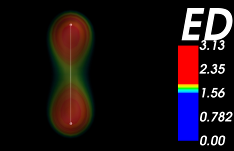
A further example plotting electron density around a water molecule within Mayavi can be found here.