Statistics of small samples: hypothesis testing and correlation

Nov 2005/07/08/11

This set of notes focuses on hypothesis testing and correlation with small-sized samples. We assume you are generally familiar with topics in probability and statistics, including:

¶ Definition of probability
¶ Probability distribution, probability density function = pdf
¶ Random variable
¶ Independent events vs "chains of events": states of a baseball game...
¶ Expectation...average?
¶ permutations vs combinations
¶ Number of combinations of N things taken r at a time
¶ Normal distribution, binomial distribution, Poisson distribution
¶ Variance and standard deviation
¶ normalizing a data point x to z by subtracting the mean and dividing by the standard deviation

Binomial distribution example in Matlab and EXCEL:
Suppose the probability that someone is left-handed is 0.1 = p.
What is the probability that NO people out of a SAMPLE of 10 are left-handed?
0.9^10 = 35%
in general, if r is the number of left handers in a sample of N, type into the command line:
>> r=0; N = 10; p = 0.1; q = 1-p;

typed on Matlab command line:
probL = q^(N-r)*p^r*nchoosek(r, N)
or EXCEL function =BINOMDIST(r, N, p, 0);

Knowing from EXCEL help that
BINOMDIST(number_s, trials, probability_s, cumulative)
type into an EXCEL cell
=BINOMDIST(0, 10, 0.1, 0)
to see the answer 0.34867844 ~ 35%

The standard deviation of a binomial distribuiton = sqrt(p*q*n) where n = number of trials (coin flips)

Computing factorial and number of combinations:
EXCEL: fact, combin...Matlab factorial(N), nchoosek(N, r)
fact(200) too big for EXCEL, but not combin(200, 20)...
However combin(2000, 500) is too big for EXCEL

365 is such a large number...
for thinking about the same-birthday problem
any 2 of N have 1/365 chance of sharing same day...
combin(N, 2) > 180 results for N = 20
different answer of 23 from http://en.wikipedia.org/wiki/Birthday_problem
human birth season, twins...
result for EN123 student pop?

Poisson distribution from Binomial, appropriate for very low p.

See application in Katz, 1959, for Nobel Prize in 1970

epsp = "excitatory post-synaptic potential". 78 spontaneous epsps were observed, and had an averge peak of 0.4mV. In the link above see Figs 5 and 6; the histograms there are the result of 198 single nerve impulses (presynaptic) spaced several seconds apart. Of the 198 impulses 19 resulted in NO epsp (failure). Fig 5 is reproduced in Katz' book Nerve, Muscle and Synapse (1966, McGraw-Hill) on page 137; on page 135 he compiles the following numbers by adding up the 3 histogram bars near each of the peaks:
18 failure
44 0.4 mV peak
55 0.8 mV peak
36 1.2 mV
25 1.6 mV
12 2.0 mV
5  2.4
2  2.8
1  3.2
0  3.6
These data are well fit by a Poisson n*p = 2.3, the only free parameter in the equation. What is n in n*p? Not 198, the number of shocks to the presynaptic axon. It turns out n is the number of vesicles in the presynaptic synapse. See figure below, from basal ganglia (research of Tepper, from Rutgers...)

How many vesicles are there per synapse? Anywhere from hundreds to thousands. One estimate says 987 vesicles per cubic micron. There are docking vesicles, ready to be released, and reserve vesicles, recently reconstituted, away from the membrane facing the synpatic cleft. At any rate, p is the probability that one vesicle will be released (due to one stimulation shock...)

2011: What happens in a direct test of the Katz data with the binomial distribution? n is the number of vesicles in the synapse and p is probability of release of one vesicle from one presynaptic "shock." Want n^p = 2.3. Use Excel to find
=binomdist(0, 100, 0.023, 0) = .0976015 ; *198 = 19 (rounded off...)
=binomdist(0, 200, 0.0115, 0) = .0988315
=binomdist(0, 400, 0.00575, 0) = .0995955
as long as n*p = 2.3 it is basically verified that the Poisson approx is correct... who needs Poisson?

try = BINOMDIST(2, 100, 0.023, 0) * 198 = 53, close to 55

Is such a skewed distribution (long tail) normal? No. Only when p = 0.5 does a binomial distribution look normal and symmetric.

The Katz' results plus electron micrographic images of vesicles, are taken as solid evidence that there is a quantal nature to the release of neurotransmitter, from vesicles, each vesicle containing nearly the same number of transmitter molecules.

example in EXCEL: 2.33/198 = .0117 and
=POISSON(0, 0.0117*198, 1) gives 0.097 and 0.097*198 = 19
=BINOMDIST(0, 198, .0117, 1) gives0.097 also.
since we're looking at 0 events, =BINOMDIST(0, 198, .0117, 0) would give the same answer since the 4th input argument is a flag for cumulative(1) or not (0)...
%--------------- ---------------

if p is closer to 0.5, then the normal distribution approx is

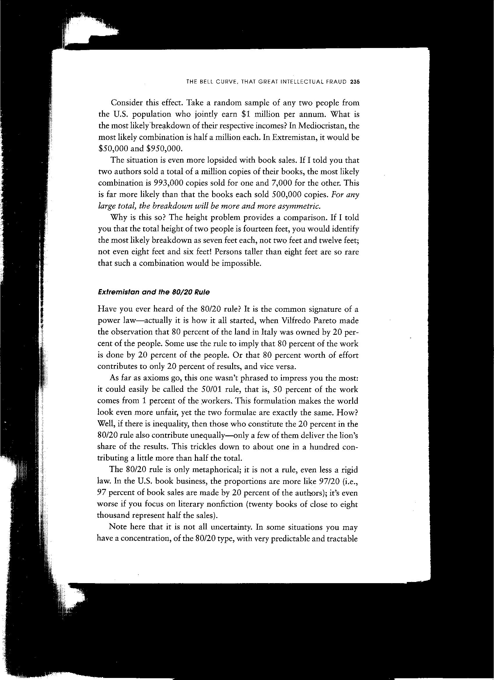
2008: Nicholas Taleb: Black Swan events; see page 235 from the book: What is the underlying power law?
Suppose 100 people own land in Italy, and you order and number them from least to most.
the following matlab script gives frac 21% owned by the first 80%
(yes, the integral of the power fcn could be used...)
Occupy Italy?

2012: Men's height: over 7 feet... Women's height: shorter than normal
--------------------------------------------

Some of the material for this file has been inspired by reading Chapters 7-10 of Loftus & Loftus, Essence of Statistics, 2nd Ed (Knopf, 1988).

Hypothesis Testing: Before we look at the details of calculating probabilities and making decisions, examine the Table below to appreciate the 4 possibilities relating reality to prediction. The null hypothesis is the status quo, it means the new idea is wrong, the defendant is innocent. No news. The alternative hypothesis is your new idea, an explanation for data that defies the conventional wisdom.

Mistakenly rejecting the null hypothesis (false positive) is the worst mistake; it means you judge that some "new" cause-effect relationship has been discovered, and you're likely to inspire other researchers to follow up. Like finding an innocent man guilty.

More detail: Some independent variable has been changed in the experiment and the data is the dependent variable. The null hypothesis is that the independent variable has no affect on the dependent variable. You want to test that hypothesis.

Rejecting the null hypothesis means that your experiment supports the idea that the independent variable affects the dependent variable. Say the independent variable is blood-alcohol-concentration (BAC) and the dependent variable is max frequency of rotation of a knob. Each subject is tested sober and inebriated, resulting in two lists of numbers, to be processed by a t-test, with a criterion for significance to meet.

2011: Signal detection theory SDT ; started by Green and Swets (1966)
http://wise.cgu.edu/sdtmod/index.asp
appropriate topic for EN123 as SDT considers the detection of faint signals.

http://teachline.ls.huji.ac.il/72633/SDT_intro.pdf
Heeger (NYU) Lecture notes:
Consider a difficult-to-detect "signal" (say tumor in CT scan) for a radiologist/detector: 4 possibilities:

Information vs Criterion: "...some doctors may feel that missing an opportunity for early diagnosis may mean the difference between life and death. A false alarm, on the other hand, may result only in a routine biopsy operation. They may choose to err toward yes (tumor present) decisions. Other doctors, however, may feel that unnecessary surgeries (even routine ones) are very bad (expensive, stress, etc.). They may chose to be more conservative and say no (no turmor) more often. They will miss more tumors, but they will be doing their part to reduce unnecessary surgeries. And they may feel that a tumor, if there really is one, will be picked up at the next check-up. These arguments are not about information. Two doctors, with equally good training, looking at the same CT scan, will have the same information. But they may have a different bias/criterion."

External and and internal noise--internal to the detector/observer.

"...the proportions of Hits and FAs reflect the effect of two underlying parameters: the first one reflects the separation between the signal and the noise (d') and the second one the strategy of the participant (C)." (Adbi)

Decision strategy: Pick a criterion along the detector-response axis (signal + noise) and responses above that criterion call for Hit. Low criterion will result in more false positives.

Receiver Operating Characteristic ROC The "discriminability" d' curves. false alarm on H axis, Hits on V axis.

d' = separation / spread

One goal of SDT: estimate d' and criterion from hits and false alarm rates. see wise.cgu.edu site.

Legal example: As a defense lawyer you'd like the jury to return a "not guilty" verdict. Implying you'd like to seat conservative jurors who require considerable evidence of guilt before "detecting the guilty signal."

College example: Cynical students may select professors who require little evidence that someone deserves an A. A low "criterion value for detecting that A aura" signal from a student...

--------------------------------------------

The other kind of sampling:
What it means to "draw a sample from a distribution": The (probability) distribution represents the population as a whole from which the sample is drawn. Ideally you would know the mean and standard deviation of the population. Your concern make the size of the sample large enough to test your hypothesis, but not so large as to be too expensive or time consuming. (How many people to call overnight in a political poll...)

The 2-tail/1-tail "paradox". Suppose you are testing the hypothesis that guesses as to my correct weight may be either too small or too large. I know my exact weight, but don't know the standard deviation of all guesses, only the s.t.d. of, say, a sample of 6 guesses. Form a data set of the differences (positive or negative) between the guesses and my actual weight. Estimate the variance of the population from

Next divide the est. variance by N=6 to find the est. variance of the means of sample size 6.

The null hypothesis, at a 95% criterion, would be that 95% of the mean guesses fall between 2.5% less and 2.5% more. Suppose the result is that in the one sample you have, the mean is large enough that it is greater than 97% of size-6 guess means. By the 2-tail criteria, the alt. hypothesis fails. But suppose you now change your hypothesis to say that guesses to my weight will be greater than actual. OK, your alt hypothesis succeeds at the 5% level. But you have now changed your mind...something that perhaps wasn't known by a reviewer approving your process.

Example: The school that wants to admit students with SATs above one level but below another level (to insure good students on one hand and to have a good "selectivity" rating on the other hand: don't admit students that are just going to go somewhere else...)

The paradox is resolved by being clear about what the alt hypothesis is before starting analysis. n.b.: one section of the SAT is arranged to have a mean of 500 and a standard deviation of 100. Grading on the curve: a score 2 std_dev above avg receives an A; one std_dev greater, a B.

Blind experimenters: We the scientific establishment don't want you the experimenter testing subjects you know to be in the "alt hypothesis" group; you would be too biased in favor of your hypothesis: better for a third party to select your subjects and give them either the drug or the placebo, or put them in the normal environment or the all-vertical striped drum...

Are you smarter than a 10th grader? Sample of one: Suppose you score 600 on the SAT math test, knowing average 10th grader scores 500. What's the probability that you're smarter than a 10th grader? Well, you did get a higher score, by one standard deviation, and
=NORMDIST(600, 500, 100, 1) = 0.84, and 1-0.84 = 16% the one-tailed probability that someone will score 600 or more. You're in the 84th percentile.

That's all that can be said; one POV: it would not make much sense for you to take the test again, you might do better the second time just because of the practice.

1. Considering whether a sample has been drawn from the distribution of a population. The population mean and variance are known. For example from the population of all current Brown Univ students we may know that the average SAT verbal score was 700 with a standard deviation of 60. We have a sample of 20 left-handed Brown students who have an average SAT verbal score of 720.

What we are really concerned with is the distribution of means of all samples of size 10 drawn from the population. It turns out that the variance of the sample-size-N distribution can be calculated (more precisely the formula below can be proved as a theorem), and the answer is

where N is the size of the sample and σ^2_M is the variance of the distribution of samples size N drawn from the population.

Suppose, as you saw above, if the sample size were N=1; then we would end up with the "sample" σ equal to the population σ now suppose the size of the samples were equal to the population, then the variance of the means would be zero, because all means would be the same. So the idea seems reasonable, about dependence of σ on sqrt of N.

Once we have the variance of the means-of-sample-size-N distribution, we can calculate a z term,

In the old days the value of z would be looked up in a table of a normalized normal distribution; the table would tell what the integral from -∞ to z is, and we would draw conclusions from that reading.

Nowadays we can use EXCEL function NORMDIST: NORMDIST(mu_samp, mu_pop, samp_standard_dev, integral=TRUE) .

We don't really need to calculate z; just give NORMDIST the sample mean, population mean, sample s.t.d. and say you want the cumlative integral from of answer (not the "point-on-curve" calculation).

For the example above, type into an EXCEL cell =NORMDIST(720, 700, 60/sqrt(20), TRUE) hit enter, and see the answer 0.932 appear.

What does the answer mean? That 93% of samples-size-20 drawn from the Brown SAT-verbal distribution have a mean less than 720. But if your criterion for accepting a significant difference is 95% (or 5% of the tail) then you would need a larger sample to confirm that...what? Your alternative hypothesis that left hand students at Brown are drawn from a different distribution, one that has significantly higher SAT verbal scores. Another way of stating the result: that you are 93% confident that left-handers at Brown have higher SAT-verbal scores. Yet another way of interpreting the 93% answer: At the 7% level you reject the null hypothesis that there is no difference between the population as a whole and left-handed students in regard to SAT-verbal score.

How large of a sample would be needed to be at the 95% confidence level, assuming the sample average stays at 720? Answer, by trial-and-error in EXCEL: N = 25.

%----------------- --------------------

Digression for election day: Errors in polling errors: A qualifier seen in news articles about political polling: margin of error: 3.1% margin of error: Suppose X voters out of N sampled will vote for your candidate. What is the number of voters N needed in a sample to insure that 95% of the time the actual percentage of voters underlying your candidate's percentage of X/N will be within ±3.1 percent of X/N? This question, whose answer is N=1000 and whose derivation is here, is different from the question (answered below): What should be N so that you're confident at the 95% level that the range of poll percentages is ±3 percent of X/N if you repeated the poll many times?

The result can be tested by using matlab to simulate many polls of size 4270 and looking at the range of percentages, then finding out what fraction of the many polls are within 3% of X/N.
See [signif, mat_sort] = SampSizeTest05(samp_num, test_num) in work\fold23

See NormVoteStat08.xls for a direct test that candidate C has 95% confidence that he will win. What polling percentage will he need? It will depend on how many are in the sample...

% ------------ ------------------

2. Comparing two variants of a population: We looked at whether an experimental group within a population is significantly different... Now what about comparing two experimental groups of a known population compared with each other? Left-handed males, and left-handed females, for example.

You will form a z term of difference of means:

Where S1 and S2 are the two samples to be compared. Notice the two estimated variances are added together

Suppose it's known that the average area of maple leaves on the ground in October is 25 cm-sq, with a standard deviation of 5 cm-sq. A sample of 12 Japanese maple leaves has an averge area of 34 cm-sq. Someone else comes in with a sample of 18 big leaf maple leaves with an average area of 38 cm-sq. Is it significant at the 5% level that big leaf maple leaves are larger than Japanese maple leaves?
From the above formula, the estimated std_dev is 1.86, z is 2.14 and =NORMDIST(4, 0, 1.86, 1) = 0.984,
so the significance is 1.6% < 5% answer: yes the difference is signifcant.
Big Leaf Maple leaves

3. If population statistics are not available:
Now suppose, like in the case of the Lab 9 knob rotation experiment, with 11 subjects, that population statistics are not known.
What can be done with s.t.d. of the samples? In their chpt 9, on parameter estimation, Loftus & Loftus say that with sample variance S^2 then

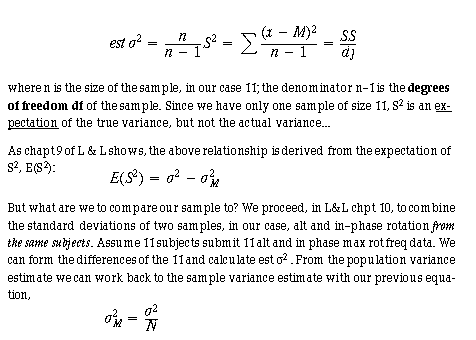
The resulting standard_dev can be divided into a difference, greater than zero, but we should not call it a z variable, but a t-variable.
What is t? From Adler & Roessler, Intro to Prob & Stat 5th Ed, Freeman (1972), p. 156,

Where m is the "null hypothesis mean" of the population.
The distribution of t depends on n and is available in tables or
kept as a calculation in EXCEL of TDIST(t, degrees of freedom, tails)
expressed as a cumulative probability.

For example, suppose a sample of 9 femurs from ring-tailed lemurs show their mean length to be 20 cm, And that the variance of the length is 9 cm. What is the probability that the ringtail lemur femurs are NOT from a population of mean length 24 cm?

ring-tailed lemur from Madagascar

4. Comparing two samples of different size, without knowing population stats: (like the knob rotation problem) In this case the degrees of freedom is n1 + n2 - 2, where n1 is the size of sample 1 and n2 is the size of sample 2. The variance of the sample means for this problem is the sum of the two sample variances of the two means. Then term m in the t-test formula above is normally set to 0, so

where the variances are of the sample means.

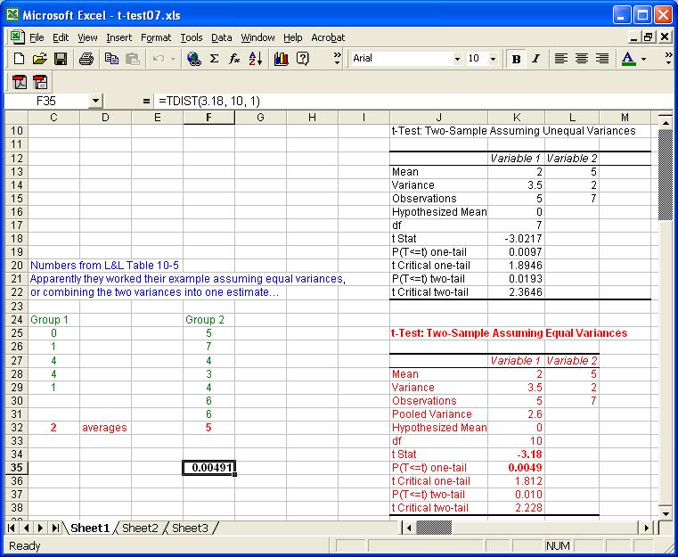
(2007) Two small samples of different sizes, with different variances: Example 10-5 from L&L: In the notes handed out, you can study an example whose data base is reproduced below in a screen shot of an EXCEL spreadsheet. There are two samples, one of 5 subjects and the other of 7 subjects. As you can see, the L&L analysis ends up with a t value of 3.18. If you look under EXCEL/Tools/Data Analysis near the bottom of the menu are two choices, "t-Test: Two Sample Assuming Equal Variances" and "t-Test: Two Sample Assuming Unequal Variances." If you run these tools on the Example 10-5 data only the "equal variances" choice comes up with the same t answer of 3.18. As you follow the Loftus and Loftus method, you see they combine two unequal variances into a weighted single variance.

Notice that in the cell highlighted below TDIST is used to calculate the one-tailed probability associated with the t-value of 3.18 and 10 degrees of freedom.

For the knob rotation lab you can use the "t-Test: Paired Two Sample for Means" tool.

Creating your own data sample of given mean and standard deviation: The pdf, probability density function, is the integral of the probability distribution. What happens if you sample at equal intervals of cumulative probability increase, and pick off the associated z values, then un-normalize them? See test code in folder fold23 function [pdfx, pdfy, samp] = pdf_tst08(div, mu, stdv) (2008). The result will be a sample with a smaller variance than the underlying population, as mentioned above.

Correlation. In hypothesis testing with t-test we are interested in how different one group is from another. Correlation looks at how similar one set of data is to another. Must be "paired data".

Example: In the knob rotation lab we record from the same subject the max rotation frequency for the dominant and the non-dominant hands. Results vary from subject to subject. Are the results correlated? (is the Dom/ND ratio always the same for each subject?)

Definition of correlation: Assume we have a set of paired data { x, y }


Example: a list of numbers correlated with itself will have an r value of 1.0. Some of the pairs will have products greater than 1, but because of mean = 0, most will have products less than 1. The average of the pairs will be 0, the sum will be M-1, and the r value (M-1)/(M-1) = 1.

The correlation coefficient will be between -1 and +1.
A correlation of zero means the two variables are independent. A correlation near -1 means the two variables related with a minus sign factor, Y = -m*X...

A threshold can be set to determine if correlation meets a criterion: greater than 0.5 for example.

Graphics: plot y data vs x data and look for the points to lie on a straight line for perfect correlation, either plus or minus.

In EXCEL you can find the operation Pearson: from the EXCEL Help menu we learn that it
Returns the Pearson product moment correlation coefficient, r, a dimensionless index that ranges from -1.0 to 1.0 inclusive and reflects the extent of a linear relationship between two data sets.

Syntax

PEARSON(array1,array2)

Array1 is a set of independent values.

Array2 is a set of dependent values.

A B
9 10
7 6
5 1
3 5
1 3
Formula Description (Result)
=PEARSON(A2:A6,B2:B6)
Pearson product moment correlation coefficient for the data sets above (0.699379)

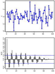
Extra: Shifting time series to match up cause and effect; cross-correlation;
special case of auto-correlation. See image below, from wikipedia, of a time series with a hidden sine wave, and the autocorrelation that reveals the hidden pattern...

Glossary/Summary:
null hypothesis: 2x2 matrix of decision vs reality
number of combinations of N things taken r at at time
binomial distribution
normal (gaussian, bell curve) distribution
Poisson distribution: release of synaptic vesicles example
standard deviation of samples of size N
estimating variance when population stats not available
when to use t-test and t tables
EXCEL functions NORMDIST, BINOMDIST, TDIST, POISSON, COMBIN
use of EXCEL Data Analysis Toolbox for statistics
Correlation, cross correlation

extra:
Fuzzy Logic, fuzzy membership in fuzzy sets: To what degree is someone in the fuzzy set of tall people?
Curse of Dimensionality
Baseball batting order optimization (Markov chain, conditional probabilities)
See RS vs TB sheet
states 0, 1, 2 outs; runners on nowhere, 1, 1-2, 1-3, 2-3, 1-2-3 implies 18 states.
What's the probability of changing from one state to another, and is a run-scored during that state transition?

for nn = 1:100
ara(nn) = nn^6; % the power is 6
end,
tot = sum(ara);
tot80 = sum(ara(1:80);
frac = tot80/tot

but
tot98 = sum(ara(1:98))
and
tot98/frac = 86%, so the top 2% do not own 50% of the land...