Chapter 5

 

Vibrations

 

 

 

5.1 Overview of Vibrations

 

 

5.1.1 Examples of practical vibration problems

 

Vibration is a continuous cyclic motion of a structure or a component.

 

Generally, engineers try to avoid vibrations, because vibrations have a number of unpleasant effects:

·         Cyclic motion implies cyclic forces.  Cyclic forces are very damaging to materials.

·         Even modest levels of vibration can cause extreme discomfort;

·         Vibrations generally lead to a loss of precision in controlling machinery.

 

Examples where vibration suppression is an issue include:

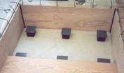
Structural vibrations.  Most buildings are mounted on top of special rubber pads, which are intended to isolate the building from ground vibrations.  The figure on the right shows vibration isolators being installed under the floor of a building during construction (from www.wilrep.com )

 

No vibrations course is complete without a mention of the Tacoma Narrows suspension bridge.  This bridge, constructed in the 1940s, was at the time the longest suspension bridge in the world.  Because it was a new design, it suffered from an unforseen source of vibrations.  In high wind, the roadway would exhibit violent torsional vibrations, as shown in the picture below.

 

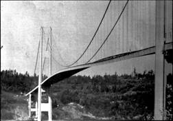
You can watch newsreel footage of the vibration and even the final collapse at http://www.youtube.com/watch?v=HxTZ446tbzE  To the credit of the designers, the bridge survived for an amazingly long time before it finally failed.  It is thought that the vibrations were a form of self-excited vibration known as `flutter,’ or ‘galloping’  A similar form of vibration is known to occur in aircraft wings.  Interestingly, modern cable stayed bridges that also suffer from a new vibration problem: the cables are very lightly damped and can vibrate badly in high winds (this is a resonance problem, not flutter). You can find a detailed article on the subject at www.fhwa.dot.gov/bridge/pubs/05083/chap3.cfm. Some bridge designs go as far as to incorporate active vibration suppression systems in their cables.

 

 

 

 

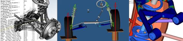
Vehicle suspension systems are familiar to everyone, but continue to evolve as engineers work to improve vehicle handling and ride (the figure above is from http://www.altairhyperworks.com.   A radical new approach to suspension design emerged in 2003 when a research group led by Malcolm Smith at Cambridge University invented a new mechanical suspension element they called an ‘inerter’.   This device can be thought of as a sort of generalized spring, but instead of exerting a force proportional to the relative displacement of its two ends, the inerter exerts a force that is proportional to the relative acceleration of its two ends.  An actual realization is shown in the figure.  You can find a detailed presentation on the theory behind the device at http://www-control.eng.cam.ac.uk/~mcs/lecture_j.pdf The device was adopted in secret by the McLaren Formula 1 racing team in 2005 (they called it the ‘J damper’, and a scandal erupted in Formula 1 racing when the Renault team managed to steal drawings for the device, but were unable to work out what it does.   The patent for the device has now been licensed Penske and looks to become a standard element in formula 1 racing.  It is only a matter of time before it appears on vehicles available to the rest of us.

 

Precision Machinery: The picture on the right shows one example of a precision instrument.   It is essential to isolate electron microscopes from vibrations.  A typical transmission electron microscope is designed to resolve features of materials down to atomic length scales.  If the specimen vibrates by more than a few atomic spacings, it will be impossible to see!  This is one reason that electron microscopes are always located in the basement $–$ the basement of a building vibrates much less than the upper floors.   Professor K.-S. Kim at Brown recently invented and patented a new vibration isolation system to support his atomic force microscope on the 7^th floor of the Barus-Holley building $–$ you can find the patent at United States Patent, Patent Number 7,543,791.

 

Here is another precision instrument that is very sensitive to vibrations.

 

 

 

 

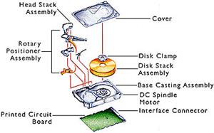The picture shows features of a typical hard disk drive.  It is particularly important to prevent vibrations in the disk stack assembly and in the disk head positioner, since any relative motion between these two components will make it impossible to read data. The spinning disk stack assembly has some very interesting vibration characteristics (which fortunately for you, is beyond the scope of this course).

 

 

 

 

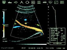Vibrations are not always undesirable, however.  On occasion, they can be put to good use.  Examples of beneficial applications of vibrations include ultrasonic probes, both for medical application and for nondestructive testing. The picture shows a medical application of ultrasound: it is an image of someone’s colon.  This type of instrument can resolve features down to a fraction of a millimeter, and is infinitely preferable to exploratory surgery.  Ultrasound is also used to detect cracks in aircraft and structures.

 

Musical instruments and loudspeakers are a second example of systems which put vibrations to good use.  Finally, most mechanical clocks use vibrations to measure time. 

 

 

5.1.2 Vibration Measurement

 

When faced with a vibration problem, engineers generally start by making some measurements to try to isolate the cause of the problem.  There are two common ways to measure vibrations:

 

1.      An accelerometer is a small electro-mechanical device that gives an electrical signal proportional to its acceleration.   The picture shows a typical 3 axis MEMS accelerometer (you’ll use one in a project in this course).   MEMS accelerometers should be selected very carefully $–$ you can buy cheap accelerometers for less than $50, but these are usually meant just as sensors, not for making precision measurements.   For measurements you’ll need to select one that is specially designed for the frequency range you are interested in sensing.  The best accelerometers are expensive ‘inertial grade’ versions (suitable for so-called ‘inertial navigtation’ in which accelerations are integrated to determine position) which are often use Kalman filtering to fuse the accelerations with GPS measurements.

 

2.      A displacement transducer is similar to an accelerometer, but gives an electrical signal proportional to its displacement.

 

Displacement transducers are generally preferable if you need to measure low frequency vibrations; accelerometers behave better at high frequencies.

 

 

 

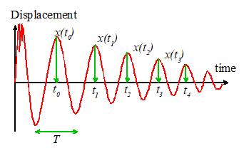
5.1.3  Features of a Typical Vibration Response

The picture below shows a typical signal that you might record using an accelerometer or displacement transducer.

 

Important features of the response are

 

       The signal is often (although not always) periodic: that is to say, it repeats itself at fixed intervals of time.  Vibrations that do not repeat themselves in this way are said to be random.  All the systems we consider in this course will exhibit periodic vibrations.

 

       The PERIOD  of the signal, T,  is the time required for one complete cycle of oscillation, as shown in the picture.

 

        The FREQUENCY of the signal, f,  is the number of cycles of oscillation per second. Cycles per second is often given the name Hertz: thus, a signal which repeats 100 times per second is said to oscillate at 100 Hertz.

 

        The ANGULAR FREQUENCY of the signal, $\omega$, is defined as $\omega =2\pi f$. We specify angular frequency in radians per second.  Thus, a signal that oscillates at 100 Hz has angular frequency $200\pi$ radians per second.

 

       Period, frequency and angular frequency are related by

 

$f=\frac{1}{T}\omega =2\pi f=\frac{2\pi }{T}$

 

 

       The PEAK-TO-PEAK AMPLITUDE of the signal, A, is the difference between its maximum value and its minimum value, as shown in the picture

 

        The AMPLITUDE of the signal is generally taken to mean half its peak to peak amplitude. Engineers sometimes use amplitude as an abbreviation for peak to peak amplitude, however, so be careful.

 

        The ROOT MEAN SQUARE AMPLITUDE or RMS amplitude is defined as

$\sigma ={\left\{\frac{1}{T}{\displaystyle \underset{0}{\overset{T}{\int }}{\left[y(t)\right]}^2}dt\right\}}^{1/2}$

 

 

 

 

 

 

5.1.4  Harmonic Oscillations

 

 Harmonic oscillations are a particularly simple form of vibration response.  A conservative spring-mass system will exhibit harmonic motion $–$ if you have Java, Internet Explorer (or a browser plugin that allows you to run IE in another browser) you can run a Java Applet to visualize the motion.  You can find instructions for installing Java, the IE plugins, and giving permission for the Applet to run here.  The address for the SHM simulator (cut and paste this into the Internet Explorer address bar)

http://www.brown.edu/Departments/Engineering/Courses/En4/java/shm.html

If the spring is perturbed from its static equilibrium position, it vibrates (press `start’ to watch the vibration).  We will analyze the motion of the spring mass system soon. We will find that the displacement of the mass from its static equilibrium position, $x$, has the form

$x(t)=\Delta X\sin (\omega t+\varphi )$

Here, $\Delta X$ is the amplitude of the displacement, $\omega$ is the frequency of oscillations in radians per second, and $\varphi$ (in radians) is known as the `phase’ of the vibration.  Vibrations of this form are said to be Harmonic. 

 

Typical values for amplitude and frequency are listed in the table below

 

 

We can also express the displacement in terms of its period of oscillation T

$x(t)=\Delta X\sin \left(\frac{2\pi }{T}t+\varphi \right)$

 

The velocity $v$ and acceleration $a$ of the mass follow as

$\begin{array}{l}v(t)=\Delta V\sin \left(\omega t+\varphi \right)V_0=\omega \Delta X\cos \left(\omega t+\varphi \right)\\ a(t)=-\Delta A\sin \left(\omega t+\varphi \right)\Delta A=\omega \Delta V={\omega }^2\Delta X\end{array}$

 

Here, $\Delta V$ is the amplitude of the velocity, and $\Delta A$ is the amplitude of the acceleration.  Note the simple relationships between acceleration, velocity and displacement amplitudes.

 

Surprisingly, many complex engineering systems behave just like the spring mass system we are looking at here.  To describe the behavior of the system, then, we need to know three things (in order of importance):

(1) The frequency (or period) of the vibrations

(2) The amplitude of the vibrations

(3) Occasionally, we might be interested in the phase, but this is rare.

 

So, our next problem is to find a way to calculate these three quantities for engineering systems.

 

We will do this in stages.  First, we will analyze a number of freely vibrating, conservative systems.  Second, we will examine free vibrations in a dissipative system, to show the influence of energy losses in a mechanical system.  Finally, we will discuss the behavior of mechanical systems when they are subjected to oscillating forces.

 

5.2 Free vibration of conservative, single degree of freedom, linear systems.

 

First, we will explain what is meant by the title of this section.

       Recall that a system is conservative if energy is conserved, i.e. potential energy + kinetic energy = constant during motion.

       Free vibration means that no time varying external forces act on the system. 

       A system has one degree of freedom if its motion can be completely described by a single scalar variable.  We’ll discuss this in a bit more detail later.

        A system is said to be linear if its equation of motion is linear.  We will see what this means shortly.

 

It turns out that all 1DOF, linear conservative systems behave in exactly the same way.  By analyzing the motion of one representative system, we can learn about all others.

 

We will follow standard procedure, and use a spring-mass system as our representative example.

 

 

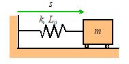
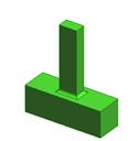
Problem:  The figure shows a spring mass system.  The spring has stiffness k and unstretched length $L_0$.  The mass is released with velocity $v_0$ from position $s_0$ at time $t=0$.  Find $s(t)$.

 

There is a standard approach to solving problems like this

 

(i) Get a differential equation for s using F=ma (or other methods to be discussed)

(ii) Solve the differential equation.

 

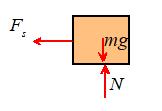
The picture shows a free body diagram for the mass.

 

 Newton’s law of motion states that

$F=ma\Rightarrow -F_{s}i+(N-mg)j=m\frac{d^{2}s}{d{t}^2}i$

The spring force is related to the length of the spring by $F_s=k(s-L_0)$.  The i component of the equation of motion and this equation then shows that

$m\frac{d^{2}s}{d{t}^2}+ks=k{L}_0$

This is our equation of motion for s.

 

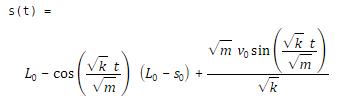
Now, we need to solve this equation.  We could, of course, use Matlab to do this $–$ in fact here is the Matlab solution.  

syms m k L0 s0 v0 real
syms v(t) s(t)
assume(k>0); assume(m>0);
diffeq = m*diff(s(t),t,2) + k*s(t) == k*L0;
v(t) = diff(s(t),t);
IC = [s(0)==s0, v(0)==v0];
s(t) = dsolve(diffeq,IC)

In practice we usually don’t need to use matlab (and of course in exams you won’t have access to matlab!)

 

 

 

5.2.1 Using tabulated solutions to solve equations of motion for vibration problems

 

Note that all vibrations problems have similar equations of motion.  Consequently, we can just solve the equation once, record the solution, and use it to solve any vibration problem we might be interested in.  The procedure to solve any vibration problem is:

1.      Derive the equation of motion, using Newton’s laws (or sometimes you can use energy methods, as discussed in Section 5.3)

2.      Do some algebra to arrange the equation of motion into a standard form

3.      Look up the solution to this standard form in a table of solutions to vibration problems.

 

We have provided a table of standard solutions as a separate document that you can download and print for future reference.   Actually, this is exactly what MATLAB is doing when it solves a differential equation for you $–$ it is doing sophisticated pattern matching to look up the solution you want in a massive internal database.

 

We will illustrate the procedure using many examples.

 

5.2.2 Solution to the equation of motion for an undamped spring-mass system

 

We would like to solve

$m\frac{d^{2}s}{d{t}^2}+ks=k{L}_0$

with initial conditions  $\frac{ds}{dt}=v_0$ from position $s_0$ at time $t=0$.

 

We therefore consult our list of solutions to differential equations, and observe that it gives the solution to the following equation

$\frac{1}{{\omega }_n^2}\frac{d^{2}x}{d{t}^2}+x=C$

 

This is very similar to our equation, but not quite the same.  To make them identical, divide our equation through by k  

$\frac{m}{k}\frac{d^{2}s}{d{t}^2}+s=L_0$

We see that if we define

$\frac{m}{k}=\frac{1}{{\omega }_n^2}\Rightarrow {\omega }_n=\sqrt{\frac{k}{m}}x=sC=L_0$

then our equation is equivalent to the standard one.

 

HEALTH WARNING: it is important to note that this substitution only works if $L_0$ is constant, so its time derivative is zero.

 

The solution for x is

$\begin{array}{c}x=C+X_0\sin \left({\omega }_{n}t+\varphi \right)\\ X_0=\sqrt{{(x_0-C)}^2+v_0^2/{\omega }_n^2}\varphi ={\tan }^{-1}\left(\frac{(x_0-C){\omega }_n}{v_0}\right)\end{array}$

Here, $x_0$ and $v_0$ are the initial value of x and $dx/dt$ its time derivative, which must be computed from the initial values of s and its time derivative

$x_0=s_0{v}_0=\frac{dx}{dt}=\frac{ds}{dt}$

 

When we present the solution, we have a choice of writing down the solution for x, and giving formulas for the various terms in the solution (this is what is usually done):

$\begin{array}{c}x=X_0\sin \left({\omega }_{n}t+\varphi \right)\\ {\omega }_n=\sqrt{\frac{k}{m}}{X}_0=\sqrt{{\left(s_0-L_0\right)}^2+v_0^2/{\omega }_n^2}\varphi ={\tan }^{-1}\left(\frac{(s_0-L_0){\omega }_n}{v_0}\right)\end{array}$

Alternatively, we can express all the variables in the standard solution in terms of  s

$s=L_0+\sqrt{{\left(s_0-L_0\right)}^2+v_0^2/{\omega }_n^2}\sin \left(\sqrt{\frac{k}{m}}t+{\tan }^{-1}\left(\frac{(s_0-L_0){\omega }_n}{v_0}\right)\right)$

But this solution looks very messy (more like the Matlab solution).

 

Observe that:

       The mass oscillates harmonically, as discussed in the preceding section;

        The angular frequency of oscillation, ${\omega }_n$, is a characteristic property of the system, and is independent of the initial position or velocity of the mass.  This is a very important observation, and we will expand upon it below.  The characteristic frequency is known as the natural frequency of the system.

         Increasing the stiffness of the spring increases the natural frequency of the system;

         Increasing the mass reduces the natural frequency of the system.

 

 

 

5.2.3 Natural Frequencies and Mode Shapes.

 

We saw that the spring mass system described in the preceding section likes to vibrate at a characteristic frequency, known as its natural frequency. This turns out to be a property of all stable mechanical systems. 

 

All stable, unforced, mechanical systems vibrate harmonically at certain discrete frequencies, known as natural frequencies of the system.

 

 

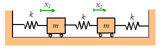
For the spring$—$mass system, we found only one natural frequency.  More complex systems have several natural frequencies.  For example, the system of two masses shown below has two natural frequencies, given by

${\omega }_1=\sqrt{\frac{k}{m}},{\omega }_2=\sqrt{\frac{3k}{m}}$

 

 

A system with three masses would have three natural frequencies, and so on.

 

In general, a system with more than one natural frequency will not vibrate harmonically.

 

For example, suppose we start the two mass system vibrating, with initial conditions

$\begin{array}{l}{x}_1={\stackrel{o}{x}}_1\frac{d{x}_1}{dt}=0\\ x_2={\stackrel{o}{x}}_2\frac{d{x}_2}{dt}=0\end{array}\}t=0$

The response may be shown (see sect 5.5 if you want to know how) to be

$\begin{array}{l}{x}_1=A_1\sin \left({\omega }_{1}t+{\varphi }_1\right)+A_2\sin \left({\omega }_{2}t+{\varphi }_2\right)\\ x_2=A_1\sin \left({\omega }_{1}t+{\varphi }_1\right)-A_2\sin \left({\omega }_{2}t+{\varphi }_2\right)\end{array}$

with

$\begin{array}{l}{A}_1=\frac{1}{2}\left(\stackrel{o}{x_1}+\stackrel{o}{x_2}\right)A_2=\frac{1}{2}\left(\stackrel{o}{x_1}-\stackrel{o}{x_2}\right)\\ {\varphi }_1=\frac{\pi }{2}{\varphi }_2=\frac{\pi }{2}\end{array}$

 

In general, the vibration response will look complicated, and is not harmonic. The animation above shows a typical example (if you are using the pdf version of these notes the animation will not work)

 

 However, if we choose the special initial conditions:

$\stackrel{o}{x_1}=X_0\stackrel{o}{x_2}=X_0$

then the response is simply

$\begin{array}{l}{x}_1=X_0\sin \left({\omega }_{1}t+{\varphi }_1\right)\\ x_2=X_0\sin \left({\omega }_{1}t+{\varphi }_1\right)\end{array}$

i.e., both masses vibrate harmonically, at the first natural frequency, as shown in the animation to the right.  

 

Similarly, if we choose

$\stackrel{o}{x_1}=X_0\stackrel{o}{x_2}=-X_0$

then

$\begin{array}{l}{x}_1=X_0\sin \left({\omega }_{2}t+{\varphi }_2\right)\\ x_2=-X_0\sin \left({\omega }_{2}t+{\varphi }_2\right)\end{array}$

i.e., the system vibrates harmonically, at the second natural frequency.

 

The special initial displacements of a system that cause it to vibrate harmonically are called  `mode shapes’ for the system.

 

If a system has several natural frequencies, there is a corresponding mode of vibration for each natural frequency.

 

The natural frequencies are arguably the single most important property of any mechanical system.  This is because, as we shall see, the natural frequencies coincide (almost) with the system’s resonant frequencies.  That is to say, if you apply a time varying force to the system, and choose the frequency of the force to be equal to one of the natural frequencies, you will observe very large amplitude vibrations.

 

When designing a structure or component, you generally want to control its natural vibration frequencies very carefully.  For example, if you wish to stop a system from vibrating, you need to make sure that all its natural frequencies are much greater than the expected frequency of any forces that are likely to act on the structure.  If you are designing a vibration isolation platform, you generally want to make its natural frequency much lower than the vibration frequency of the floor that it will stand on.  Design codes usually specify allowable ranges for natural frequencies of structures and components.

 

Once a prototype has been built, it is usual to measure the natural frequencies and mode shapes for a system.  This is done by attaching a number of accelerometers to the system, and then hitting it with a hammer (this is usually a regular rubber tipped hammer, which might be instrumented to measure the impulse exerted by the hammer during the impact).  By trial and error, one can find a spot to hit the device so as to excite each mode of vibration independent of any other.  You can tell when you have found such a spot, because the whole system vibrates harmonically.  The natural frequency and mode shape of each vibration mode is then determined from the accelerometer readings.

 

Impulse hammer tests can even be used on big structures like bridges or buildings $–$ but you need a big hammer.  In a recent test on a new cable stayed bridge in France, the bridge was excited by first attaching a barge to the center span with a high strength cable; then the cable was tightened to raise the barge part way out of the water; then, finally, the cable was released rapidly to set the bridge vibrating.

 

 

5.2.4 Calculating the number of degrees of freedom (and natural frequencies) of a system

 

When you analyze the behavior a system, it is helpful to know ahead of time how many vibration frequencies you will need to calculate.  There are various ways to do this.   Here are some rules that you can apply:

 

 

The number of degrees of freedom is equal to the number of independent coordinates required to describe the motion.  This is only helpful if you can see by inspection how to describe your system.  For the spring-mass system in the preceding section, we know that the mass can only move in one direction, and so specifying the length of the spring s will completely determine the motion of the system.  The system therefore has one degree of freedom, and one vibration frequency.   Section 5.6 provides several more examples where it is fairly obvious that the system has one degree of freedom.

 

 

For a 2D system, the number of degrees of freedom can be calculated from the equation

$n=3r+2p-N_c$

where:

$r$ is the number of rigid bodies in the system

p is the number of particles in the system

$N_c$ is the number of constraints (or, if you prefer, independent reaction forces) in the system.

 

To be able to apply this formula you need to know how many constraints appear in the problem.  Constraints are imposed by things like rigid links, or contacts with rigid walls, which force the system to move in a particular way.   The numbers of constraints associated with various types of 2D connections are listed in the table below.  Notice that the number of constraints is always equal to the number of reaction forces you need to draw on an FBD to represent the joint

 

 

 

 

For a 3D system, the number of degrees of freedom can be calculated from the equation

$n=6r+3p-N_c$

where the symbols have the same meaning as for a 2D system.   A table of various constraints for 3D problems is given below.

 

 

 

5.2.4 Calculating natural frequencies for 1DOF conservative systems

 

In light of the discussion in the preceding section, we clearly need some way to calculate natural frequencies for mechanical systems.  We do not have time in this course to discuss more than the very simplest mechanical systems.  We will therefore show you some tricks for calculating natural frequencies of 1DOF, conservative, systems. It is best to do this by means of examples.

 

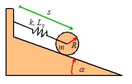
Example 1: The spring-mass system revisited

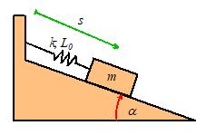
Calculate the natural frequency of vibration for the system shown in the figure. Assume that the contact between the block and wedge is frictionless.  The spring has stiffness k and unstretched length $L_0$

 

 Our first objective is to get an equation of motion for s.  We could do this by drawing a FBD, writing down Newton’s law, and looking at its components.  However, for 1DOF systems it turns out that we can derive the EOM very quickly using the kinetic and potential energy of the system. 

 

The potential energy and kinetic energy can be written down as:

$V=\frac{1}{2}k{\left(s-L_0\right)}^2-mgs\sin \alpha T=\frac{1}{2}m{\left(\frac{ds}{dt}\right)}^2$

(The second term in V is the gravitational potential energy $–$ it is negative because the height of the mass decreases with increasing s).  Now, note  that since our system is conservative

$\begin{array}{l}T+V=\text{constant}\\ \Rightarrow \frac{d}{dt}\left(T+V\right)=0\end{array}$

Differentiate our expressions for T and V (use the chain rule) to see that

$\begin{array}{l}m\frac{ds}{dt}\frac{d^{2}s}{d{t}^2}+k(s-L_0)\frac{ds}{dt}-mg\frac{ds}{dt}\sin \alpha =0\\ \Rightarrow \frac{m}{k}\frac{d^{2}s}{d{t}^2}+s=L_0+\frac{mg}{k}\sin \alpha \end{array}$

Finally, we must turn this equation of motion into one of the standard solutions to vibration equations.

Our equation looks very similar to

$\frac{1}{{\omega }_n^2}\frac{d^{2}x}{d{t}^2}+x=C$

By comparing this with our equation we see that the natural frequency of vibration is

$\begin{array}{l}{\omega }_n=\sqrt{\frac{2k}{3m}}(\text{rad/s)}\\ \text{ =}\frac{\text{1}}{\text{2}\pi }\sqrt{\frac{2k}{3m}}\left(\text{Hz}\right)\end{array}$

 

 

Summary of procedure for calculating natural frequencies:

 

(1)  Describe the motion of the system, using a single scalar variable (In the example, we chose to describe motion using the distance s);

(2) Write down the potential energy V and kinetic energy T of the system in terms of the scalar variable;

(3) Use $\frac{d}{dt}\left(T+V\right)=0$ to get an equation of motion for your scalar variable;

(4) Arrange the equation of motion in standard form;

(5) Read off the natural frequency by comparing your equation to the standard form.

 

Example 2: A nonlinear system.

 

We will illustrate the procedure with a second example, which will demonstrate another useful trick.

 

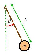
Find the natural frequency of vibration for a pendulum, shown in the figure.

We will idealize the mass as a particle, to keep things simple.

 

We will follow the steps outlined earlier:

  (1)  We describe the motion using the angle $\theta$

  (2)  We write down T and V:

$\begin{array}{l}V=-mgL\cos \theta \\ T=\frac{1}{2}m{\left(L\frac{d\theta }{dt}\right)}^2\end{array}$

(if you don’t see the formula for the kinetic energy, you can write down the position vector of the mass as $r=L\sin \theta i-L\cos \theta j$, differentiate to find the velocity: $v=L\cos \theta \frac{d\theta }{dt}i+L\sin \theta \frac{d\theta }{dt}j$, and then compute $T=m(v\cdot v)/2=m{L}^2{\left(\frac{d\theta }{dt}\right)}^2({\sin }^2\theta +{\cos }^2\theta )$ and use a trig identity.  You can also use the circular motion formulas, if you prefer).

 (3) Differentiate with respect to time:

$\begin{array}{l}m{L}^2\frac{d^2\theta }{d{t}^2}\frac{d\theta }{dt}+mgL\sin \theta \frac{d\theta }{dt}=0\\ \Rightarrow \frac{L}{g}\frac{d^2\theta }{d{t}^2}+\sin \theta =0\end{array}$

 (4) Arrange the EOM into standard form.  Houston, we have a problem.  There is no way this equation can be arranged into standard form.  This is because the equation is nonlinear ( $\sin \theta$ is a nonlinear function of $\theta$ ).  There is, however, a way to deal with this problem.  We will show what needs to be done, summarizing the general steps as we go along.

 

 

(i) Find the static equilibrium configuration(s) for the system.

 

 If the system is in static equilibrium, it does not move.  We can find values of $\theta$ for which the system is in static equilibrium by setting all time derivatives of $\theta$ in the equation of motion to zero, and then solving the equation.  Here,

$\sin {\theta }_o=0\Rightarrow {\theta }_0=0,\pi ,2\pi \mathrm{...}$

Here, we have used ${\theta }_0$ to denote the special values of $\theta$ for which the system happens to be in static equilibrium.  Note that ${\theta }_0$ is always a constant.

 

(ii) Assume that the system vibrates with small amplitude about a static equilibrium configuration of interest.

 

To do this, we let $\theta ={\theta }_0+x$, where $x<<1$.

 

Here, x represents a small change in angle from an equilibrium configuration.. Note that x will vary with time as the system vibrates.  Instead of solving for $\theta$, we will solve for x.  Before going on, make sure that you are comfortable with the physical significance of  both x and ${\theta }_0$.

 

(iii) Linearize the equation of motion, by expanding all nonlinear terms as Taylor Maclaurin series about the equilibrium configuration.

 

We substitute for $\theta$ in the equation of motion, to see that

 

$\frac{L}{g}\frac{d^{2}x}{d{t}^2}+\sin ({\theta }_0+x)=0$

(Recall that ${\theta }_0$ is constant, so its time derivatives vanish)

 

Now, recall the Taylor-Maclaurin series expansion of a function f(x) has the form

$f(x_0+x)=f(x_0)+x{f}^{\prime }(x_0)+\frac{1}{2}{x}^2{f}^{″}(x_0)+\mathrm{...}$

where

$f^{\prime }(x_0)\equiv {\frac{df}{dx}|}_{x=x_0}{f}^{″}(x_0)\equiv {\frac{d^{2}f}{d{x}^2}|}_{x=x_0}$

Apply this to the nonlinear term in our equation of motion

$\sin \left({\theta }_0+x\right)=\sin {\theta }_0+x\cos {\theta }_0-\frac{1}{2}{x}^2\sin {\theta }_0+\mathrm{...}$

Now, since x<<1, we can assume that $x^n<<x$, and so

$\sin \left({\theta }_0+x\right)\approx \sin {\theta }_0+x\cos {\theta }_0$

Finally, we can substitute back into our equation of motion, to obtain

 

$\frac{L}{g}\frac{d^{2}x}{d{t}^2}+\cos {\theta }_{0}x=-\sin {\theta }_0$

(iv) Compare the linear equation with the standard form to deduce the natural frequency.

 

We can do this for each equilibrium configuration.

${\theta }_0=0,2\pi ,4\pi \mathrm{...}\Rightarrow \frac{L}{g}\frac{d^{2}x}{d{t}^2}+x=0$

whence

$\begin{array}{l}{\omega }_n=\sqrt{\frac{g}{L}}(\text{rad/sec)}\\ f_n=\frac{1}{2\pi }\sqrt{\frac{g}{L}}(\text{Hz)}\end{array}$

Note that all these values of ${\theta }_0$ really represent the same configuration: the mass is hanging below the pivot.  We have rediscovered the well-known expression for the natural frequency of a freely swinging pendulum.

 

Next, try the remaining static equilibrium configuration

${\theta }_0=\pi ,3\pi ,5\pi \mathrm{...}\Rightarrow \frac{L}{g}\frac{d^{2}x}{d{t}^2}-x=0$

If we look up this equation in our list of standard solutions, we find it does not have a harmonic solution.  Instead, the solution is

$\begin{array}{l}x(t)=\frac{1}{2}\left(x_0+\frac{v_0}{\alpha }\right)e^{-\alpha t}+\frac{1}{2}\left(x_0-\frac{v_0}{\alpha }\right)e^{\alpha t}\\ \alpha =\sqrt{\frac{g}{L}}\end{array}$

where $x_0=x(t=0)$ and $v_0={\frac{dx}{dt}|}_{t=0}$

 

 

 

Thus, except for some rather special initial conditions, x increases without bound as time increases.  This is a characteristic of an unstable mechanical system.

 

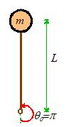
If we visualize the system with ${\theta }_0=\pi$, we can see what is happening.  This equilibrium configuration has the pendulum upside down!

 

No wonder the equation is predicting an instability…

 

Here is a question to think about.  Our solution predicts that both x and dx/dt become infinitely large.  We know that a real pendulum would never rotate with infinite angular velocity.  What has gone wrong?

 

 

 

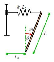
Example 3: We will look at one more nonlinear system, to make sure that you are comfortable with this procedure. Calculate the resonant frequency of small oscillations about the equilibrium configuration $\theta =0$ for the system shown. The spring has stiffness k and unstretched length $L_0$.

 

We follow the same procedure as before.

 

The potential and kinetic energies of the system are

$\begin{array}{l}V=\frac{1}{2}k{\left(L\sin \theta \right)}^2+\frac{1}{2}mgL\cos \theta \\ T=\frac{1}{2}\frac{m{L}^2}{3}{\left(\frac{d\theta }{dt}\right)}^2\end{array}$

Hence

$\begin{array}{l}\frac{d}{dt}(T+V)=\frac{m{L}^2}{3}\frac{d^2\theta }{d{t}^2}\frac{d\theta }{dt}+k{L}^2\sin \theta \cos \theta \frac{d\theta }{dt}-\frac{1}{2}mgL\sin \theta \frac{d\theta }{dt}=0\\ \Rightarrow \frac{m{L}^2}{3}\frac{d^2\theta }{d{t}^2}+\left(k{L}^2\cos \theta -\frac{mgL}{2}\right)\sin \theta =0\end{array}$

Once again, we have found a nonlinear equation of motion.  This time we know what to do.  We are told to find natural frequency of oscillation about $\theta =0$, so we don’t need to solve for the equilibrium configurations this time.  We set $\theta =0+x$, with $x<<1$ and substitute back into the equation of motion:

$\frac{m{L}^2}{3}\frac{d^{2}x}{d{t}^2}+\left(k{L}^2\cos x-\frac{mgL}{2}\right)\sin x=0$

Now, expand all the nonlinear terms (it is OK to do them one at a time and then multiply everything out.  You can always throw away all powers of x greater than one as you do so)

$\begin{array}{l}\cos x\approx 1\sin x\approx x\\ \Rightarrow \frac{m{L}^2}{3}\frac{d^{2}x}{d{t}^2}+\left(k{L}^2-\frac{mgL}{2}\right)x=0\\ \Rightarrow \frac{m}{3k\left(1-mg/2kL\right)}\frac{d^{2}x}{d{t}^2}+x=0\end{array}$

We now have an equation in standard form, and can read off the natural frequency

$\begin{array}{l}{\omega }_n=\sqrt{\frac{3k}{m}\left(1-\frac{mg}{2kL}\right)}\text{(rad/sec)}\\ f_n=\frac{1}{2\pi }\sqrt{\frac{3k}{m}\left(1-\frac{mg}{2kL}\right)}(\text{Hz)}\end{array}$

Question: what happens for $mg>2kL$?

 

Example 3: A system with a rigid body (the KE of a rigid body will be defined in the next section of the course $–$ just live with it for now!).

 

Calculate the natural frequency of vibration for the system shown in the figure.  Assume that the cylinder rolls without slip on the wedge. The spring has stiffness k and unstretched length $L_0$

 

Our first objective is to get an equation of motion for s.  We do this by writing down the potential and kinetic energies of the system in terms of s.

 

The potential energy is easy:

$V=\frac{1}{2}k{\left(s-L_0\right)}^2-mgs\sin \alpha$

The first term represents the energy in the spring, while second term accounts for the gravitational potential energy.

 

The kinetic energy is slightly more tricky.  Note that the magnitude of the angular velocity of the disk is related to the magnitude of its translational velocity by

$R\omega =\frac{ds}{dt}$

Thus, the combined rotational and translational kinetic energy follows as

$\begin{array}{l}T=\frac{1}{2}\frac{m{R}^2}{2}{\omega }^2+\frac{1}{2}m{\left(\frac{ds}{dt}\right)}^2\\ =\frac{1}{2}\frac{3m}{2}{\left(\frac{ds}{dt}\right)}^2\end{array}$

 

Now, note that since our system is conservative

$\begin{array}{l}T+V=\text{constant}\\ \Rightarrow \frac{d}{dt}\left(T+V\right)=0\end{array}$

Differentiate our expressions for T and V to see that

$\begin{array}{l}\frac{3m}{2}\frac{d^{2}s}{d{t}^2}\frac{ds}{dt}+k(s-L_0)\frac{ds}{dt}-mg\frac{ds}{dt}\sin \alpha =0\\ \Rightarrow \frac{3m}{2k}\frac{d^{2}s}{d{t}^2}+s=L_0+\frac{mg}{k}\sin \alpha \end{array}$

The last equation is almost in one of the standard forms given on the handout, except that the right hand side is not zero.  There is a trick to dealing with this problem $–$ simply subtract the constant right hand side from s, and call the result x.  (This only works if the right hand side is a constant, of course).  Thus let

$x=s-L_0-\frac{mg}{k}\sin \alpha$

and substitute into the equation of motion:

$\begin{array}{l}\frac{3m}{2k}\frac{d^{2}x}{d{t}^2}+x+L_0+\frac{mg}{k}\sin \alpha =L_0+\frac{mg}{k}\sin \alpha \\ \Rightarrow \frac{3m}{2k}\frac{d^{2}x}{d{t}^2}+x=0\end{array}$

This is now in the form

$\frac{1}{{\omega }_n^2}\frac{d^{2}x}{d{t}^2}+x=0$

and by comparing this with our equation we see that the natural frequency of vibration is

$\begin{array}{l}{\omega }_n=\sqrt{\frac{2k}{3m}}(\text{rad/s)}\\ \text{ =}\frac{\text{1}}{\text{2}\pi }\sqrt{\frac{2k}{3m}}\left(\text{Hz}\right)\end{array}$

 

 

 

5.3 Free vibration of a damped, single degree of freedom, linear spring mass system.

 

We analyzed vibration of several conservative systems in the preceding section.  In each case, we found that if the system was set in motion, it continued to move indefinitely.  This is counter to our everyday experience.  Usually, if you start something vibrating, it will vibrate with a progressively decreasing amplitude and eventually stop moving.

 

The reason our simple models predict the wrong behavior is that we neglected energy dissipation.  In this section, we explore the influence of energy dissipation on free vibration of a spring-mass system.  As before, although we model a very simple system, the behavior we predict turns out to be representative of a wide range of real engineering systems.

 

5.3.1 Vibration of a damped spring-mass system

 

The spring mass dashpot system shown is released with velocity $u_0$ from position $s_0$ at time $t=0$.  Find $s(t)$.

Once again, we follow the standard approach to solving problems like this

(i) Get a differential equation for s using F=ma

(ii) Solve the differential equation.

 

You may have forgotten what a dashpot (or damper) does.  Suppose we apply a force F to a dashpot, as shown in the figure. We would observe that the dashpot stretched at a rate proportional to the force

$F=c\frac{dL}{dt}$

One can buy dampers (the shock absorbers in your car contain dampers): a damper generally consists of a plunger inside an oil filled cylinder, which dissipates energy by churning the oil.  Thus, it is possible to make a spring-mass-damper system that looks very much like the one in the picture.  More generally, however, the spring mass system is used to represent a complex mechanical system.  In this case, the damper represents the combined effects of all the various mechanisms for dissipating energy in the system, including friction, air resistance, deformation losses, and so on.

To proceed, we draw a free body diagram, showing the forces exerted by the spring and damper on the mass.

 

Newton’s law then states that

$\begin{array}{l}k(s-L_0)+c\frac{ds}{dt}=ma=m\frac{d^{2}s}{d{t}^2}\\ \Rightarrow \frac{m}{k}\frac{d^{2}s}{d{t}^2}+\frac{c}{k}\frac{ds}{dt}+s=L_0\end{array}$

This is our equation of motion for s.

 

Now, we check our list of solutions to differential equations, and see that we have a solution to:

$\frac{1}{{\omega }_n^2}\frac{d^{2}x}{d{t}^2}+\frac{2\varsigma }{{\omega }_n}\frac{dx}{dt}+x=C$

We can get our equation into this form by setting

$s=x{\omega }_n=\sqrt{\frac{k}{m}}\varsigma =\frac{c}{2\sqrt{km}}C=L_0$

 

As before, ${\omega }_n$ is known as the natural frequency of the system.  We have discovered a new parameter, $\varsigma$, which is called the damping coefficient.  It plays a very important role, as we shall see below.

 

Now, we can write down the solution for x:

 

Overdamped System $\varsigma >1$

$x(t)=C+\exp (-\varsigma {\omega }_{n}t)\left\{\frac{v_0+(\varsigma {\omega }_n+{\omega }_d)(x_0-C)}{2{\omega }_d}\exp ({\omega }_{d}t)-\frac{v_0+(\varsigma {\omega }_n-{\omega }_d)(x_0-C)}{2{\omega }_d}\exp (-{\omega }_{d}t)\right\}$

where ${\omega }_d={\omega }_n\sqrt{{\varsigma }^2-1}$

 

Critically Damped System  $\varsigma =1$

$x(t)=C+\left\{(x_0-C)+\left[v_0+{\omega }_n(x_0-C)\right]t\right\}\exp (-{\omega }_{n}t)$

 

 

Underdamped System $\varsigma <1$

$x(t)=C+\exp (-\varsigma {\omega }_{n}t)\left\{(x_0-C)\cos {\omega }_{d}t+\frac{v_0+\varsigma {\omega }_n(x_0-C)}{\omega {}_d}\sin {\omega }_{d}t\right\}$

where ${\omega }_d={\omega }_n\sqrt{1-{\varsigma }^2}$ is known as the damped natural frequency of the system.

 

In all the preceding equations, $x_0,v_0$ are the values of x and its time derivative at time t=0.

 

These expressions are rather too complicated to visualize what the system is doing for any given set of parameters.  $–$ if you have Java, Internet Explorer (or a browser plugin that allows you to run IE in another browser) you can run a Java Applet to visualize the motion.  You can find instructions for installing Java, the IE plugins, and giving permission for the Applet to run here.  The address for the free vibration simulator (cut and paste this into the Internet Explorer address bar) is

http://www.brown.edu/Departments/Engineering/Courses/En4/java/free.html

 

You can use the sliders to set the values of either m, k, and $c$ (in this case the program will calculate the values of $\varsigma$ and ${\omega }_n$ for you, and display the results), or alternatively, you can set the values of $\varsigma$ and ${\omega }_n$ directly.  You can also choose values for the initial conditions $x_0$ and $v_0$.  When you press `start,’ the applet will animate the behavior of the system, and will draw a graph of the position of the mass as a function of time.  You can also choose to display the phase plane, which shows the velocity of the mass as a function of its position, if you wish.  You can stop the animation at any time, change the parameters, and plot a new graph on top of the first to see what has changed.  If you press `reset’, all your graphs will be cleared, and you can start again.

 

Try the following tests to familiarize yourself with the behavior of the system

       Set the dashpot coefficient $c$ to a low value, so that the damping coefficient $\varsigma <1$.   Make sure the graph is set to display position versus time, and press `start.’ You should see the system vibrate.   The vibration looks very similar to the behavior of the conservative system we analyzed in the preceding section, except that the amplitude decays with time.  Note that the system vibrates at a frequency very slightly lower than the natural frequency of the system.

       Keeping the value of $c$ fixed, vary the values of spring constant and mass to see what happens to the frequency of vibration and also to the rate of decay of vibration.  Is the behavior consistent with the solutions given above?

        Keep the values of k and m fixed, and vary $c$.  You should see that, as you increase $c$, the vibration dies away more and more quickly.  What happens to the frequency of oscillations as $c$ is increased?  Is this behavior consistent with the predictions of the theory?

        Now, set the damping coefficient (not the dashpot coefficient this time) to $\varsigma =1$.  For this value, the system no longer vibrates; instead, the mass smoothly returns to its equilibrium position x=0.  If you need to design a system that returns to its equilibrium position in the shortest possible time, then it is customary  to select system parameters so that $\varsigma =1$.  A system of this kind is said to be critically damped.

        Set $\varsigma$ to a value greater than 1.  Under these conditions, the system decays more slowly towards its equilibrium configuration.

        Keeping $\varsigma$ >1, experiment with the effects of changing the stiffness of the spring and the value of the mass.  Can you explain what is happening mathematically, using the equations of motion and their solution?

        Finally, you might like to look at the behavior of the system on its phase plane.  In this course, we will not make much use of the phase plane, but it is a powerful tool for visualizing the behavior of nonlinear systems.  By looking at the patterns traced by the system on the phase plane, you can often work out what it is doing.  For example, if the trajectory encircles the origin, then the system is vibrating.  If the trajectory approaches the origin, the system is decaying to its equilibrium configuration. 

 

 

We now know the effects of energy dissipation on a vibrating system.  One important conclusion is that if the energy dissipation is low, the system will vibrate.  Furthermore, the frequency of vibration is very close to that of an undamped system. Consequently, if you want to predict the frequency of vibration of a system, you can simplify the calculation by neglecting damping.

 

 

5.3.2 Using Free Vibrations to Measure Properties of a System

 

We will describe one very important application of the results developed in the preceding section.

 

It often happens that we need to measure the dynamical properties of an engineering system.  For example, we might want to measure the natural frequency and damping coefficient for a structure after it has been built, to make sure that design predictions were correct, and to use in future models of the system.

 

You can use the free vibration response to do this, as follows. First, you instrument your design by attaching accelerometers to appropriate points.  You then use an impulse hammer to excite a particular mode of vibration, as discussed in Section 5.1.3.  You use your accelerometer readings to determine the displacement at the point where the structure was excited: the results will be a graph similar to the one shown below.

We then identify a nice looking peak, and call the time there $t_0$, as shown.

 

The following quantities are then measured from the graph:

 

1. The period of oscillation.  The period of oscillation was defined in Section 5.1.2: it is the time between two peaks, as shown.  Since the signal is (supposedly) periodic, it is often best to estimate T as follows

$T=\frac{t_n-t_0}{n}$

where $t_n$ is the time at which the nth peak occurs, as shown in the picture.

 

 

2. The Logarithmic Decrement.  This is a new quantity, defined as follows

$\delta =\log \left(\frac{x(t_n)}{x(t_{n+1})}\right)$

where $x(t_n)$ is the displacement at the nth peak, as shown.  In principle, you should be able to pick any two neighboring peaks, and calculate $\delta$.  You should get the same answer, whichever peaks you choose.   It is often more accurate to estimate $\delta$ using the following formula

$\delta =\frac{1}{n}\log \left(\frac{x(t_0)}{x(t_n)}\right)$

This expression should give the same answer as the earlier definition.

 

Now, it turns out that we can deduce ${\omega }_n$ and $\varsigma$ from T and $\delta$, as follows.

$\varsigma =\frac{\delta }{\sqrt{4{\pi }^2+{\delta }^2}}{\omega }_n=\frac{\sqrt{4{\pi }^2+{\delta }^2}}{T}$

 

Why does this work? Let us calculate T and $\delta$ using the exact solution to the equation of motion for a damped spring-mass system.  Recall that, for an underdamped system, the solution has the form

$x(t)=\exp (-\varsigma {\omega }_{n}t)\left\{x_0\cos {\omega }_{d}t+\frac{v_0+\varsigma {\omega }_n{x}_n}{{\omega }_d}\sin {\omega }_{d}t\right\}$

where ${\omega }_d={\omega }_n\sqrt{1-{\varsigma }^2}$. Hence, the period of oscillation is

$T=\frac{2\pi }{{\omega }_d}=\frac{2\pi }{{\omega }_n\sqrt{1-{\varsigma }^2}}$

Similarly,

$\delta =\log \frac{\exp (-\varsigma {\omega }_n{t}_n)\left\{x_0\cos {\omega }_d{t}_n+\frac{v_0+\varsigma {\omega }_n{x}_n}{v_0}\sin {\omega }_d{t}_n\right\}}{\exp (-\varsigma {\omega }_n(t_n+T))\left\{x_0\cos {\omega }_d(t_n+T)+\frac{v_0+\varsigma {\omega }_n{x}_n}{v_0}\sin {\omega }_d(t_n+T)\right\}}$

where we have noted that $t_{n+1}=t_n+T$.

 

Fortunately, this horrendous equation can be simplified greatly:  substitute for T in terms of ${\omega }_n$ and $\varsigma$, then cancel everything you possibly can to see that

$\delta =\frac{2\pi \varsigma }{\sqrt{1-{\varsigma }^2}}$

 

Finally, we can solve for ${\omega }_n$ and $\varsigma$ to see that:

$\varsigma =\frac{\delta }{\sqrt{4{\pi }^2+{\delta }^2}}{\omega }_n=\frac{\sqrt{4{\pi }^2+{\delta }^2}}{T}$

as promised.

 

Note that this procedure can never give us values for k, m or $c$.  However, if we wanted to find these, we could perform a static test on the structure.  If we measure the deflection d under a static load F, then we know that

$k=\frac{F}{d}$

Once k had been found, m and $c$ are easily deduced from the relations

${\omega }_n=\sqrt{\frac{k}{m}}\varsigma =\frac{c}{2\sqrt{km}}$

 

 

5.4 Forced vibration of damped, single degree of freedom, linear spring mass systems.

 

Finally, we solve the most important vibration problems of all.  In engineering practice, we are almost invariably interested in predicting the response of a structure or mechanical system to external forcing.  For example, we may need to predict the response of a bridge or tall building to wind loading, earthquakes, or ground vibrations due to traffic.  Another typical problem you are likely to encounter is to isolate a sensitive system from vibrations.  For example, the suspension of your car is designed to isolate a sensitive system (you) from bumps in the road.  Electron microscopes are another example of sensitive instruments that must be isolated from vibrations.  Electron microscopes are designed to resolve features a few nanometers in size.  If the specimen vibrates with amplitude of only a few nanometers, it will be impossible to see!  Great care is taken to isolate this kind of instrument from vibrations.  That is one reason they are almost always in the basement of a building: the basement vibrates much less than the floors above.

 

We will again use a spring-mass system as a model of a real engineering system.  As before, the spring-mass system can be thought of as representing a single mode of vibration in a real system, whose natural frequency and damping coefficient coincide with that of our spring-mass system.

 

We will consider three types of forcing applied to the spring-mass system, as shown below:

 

External Forcing models the behavior of a system which has a time varying force acting on it.  An example might be an offshore structure subjected to wave loading.

 

Base Excitation models the behavior of a vibration isolation system.  The base of the spring is given a prescribed motion, causing the mass to vibrate.  This system can be used to model a vehicle suspension system, or the earthquake response of a structure.

 

Rotor Excitation models the effect of a rotating machine mounted on a flexible floor.  The crank with length $Y_0$ and mass $m_0$ rotates at constant angular velocity, causing the mass m to vibrate. 

 

Of course, vibrating systems can be excited in other ways as well, but the equations of motion will always reduce to one of the three cases we consider here.

 

Notice that in each case, we will restrict our analysis to harmonic excitation.  For example, the external force applied to the first system is given by

$F(t)=F_0\sin \omega t$

The force varies harmonically, with amplitude $F_0$ and frequency $\omega$. Similarly, the base motion for the second system is

$y(t)=Y_0\sin \omega t$

and the distance between the small mass $m_0$ and the large mass m for the third system has the same form.

 

We assume that at time t=0, the initial position and velocity of each system is

$x=x_0\frac{dx}{dt}=v_0$

 

In each case, we wish to calculate the displacement of the mass x from its static equilibrium configuration, as a function of time t. It is of particular interest to determine the influence of forcing amplitude and frequency on the motion of the mass.

 

We follow the same approach to analyze each system: we set up, and solve the equation of motion.

 

 

 

5.4.1 Equations of Motion for Forced Spring Mass Systems

Equation of Motion for External Forcing

 

We have no problem setting up and solving equations of motion by now.  First draw a free body diagram for the system, as show on the right

 

Newton’s law of motion gives

$m\frac{d^{2}s}{d{t}^2}=F(t)-k(s-L_0)-c\frac{ds}{dt}$

Rearrange and susbstitute for F(t)

$\frac{m}{k}\frac{d^{2}s}{d{t}^2}+\frac{c}{k}\frac{ds}{dt}+s=L_0+\frac{1}{k}{F}_0\sin \omega t$

Check out our list of solutions to standard ODEs.  We find that if we set

${\omega }_n=\sqrt{\frac{k}{m}},\varsigma =\frac{c}{2\sqrt{km}},K=\frac{1}{k}$,

our equation can be reduced to the form

$\frac{1}{{\omega }_n^2}\frac{d^{2}x}{d{t}^2}+\frac{2\varsigma }{{\omega }_n}\frac{dx}{dt}+x=C+K{F}_0\sin \omega t$ 

which is on the list.

 

The (horrible) solution to this equation is given in the list of solutions.  We will discuss the solution later, after we have analyzed the other two systems.

 

 

Equation of Motion for Base Excitation

 

Exactly the same approach works for this system.  The free body diagram is shown in the figure.  Note that the force in the spring is now k(x-y) because the length of the spring is $L_0+x-y$.  Similarly, the rate of change of length of the dashpot is d(x-y)/dt.

 

Newton’s second law then tells us that

$\begin{array}{l}m\frac{d^{2}s}{d{t}^2}=-k(s-y-L_0)-c\left(\frac{ds}{dt}-\frac{dy}{dt}\right)\\ \Rightarrow \frac{m}{k}\frac{d^{2}s}{d{t}^2}+\frac{c}{k}\frac{ds}{dt}+s=L_0+y+\frac{c}{k}\frac{dy}{dt}\end{array}$

Make the following substitutions

${\omega }_n=\sqrt{\frac{k}{m}},\varsigma =\frac{c}{2\sqrt{km}},K=1$

and the equation reduces to the standard form

$\frac{1}{{\omega }_n^2}\frac{d^{2}x}{d{t}^2}+\frac{2\varsigma }{{\omega }_n}\frac{dx}{dt}+x=C+K\left(y+\frac{2\varsigma }{{\omega }_n}\frac{dy}{dt}\right)$

Given the initial conditions

$x=x_0\frac{dx}{dt}=v_0$

and the base motion

$y(t)=Y_0\sin \omega t$

we can look up the solution in our handy list of solutions to ODEs. 

 

 

Equation of motion for Rotor Excitation

Finally, we will derive the equation of motion for the third case.  Free body diagrams are shown in the figure   for both the rotor and the mass

 

Note that the horizontal acceleration of the mass $m_0$ is

$a=\frac{d^2}{d{t}^2}(s+y)=\frac{d^{2}s}{d{t}^2}+\frac{d^{2}y}{d{t}^2}$

Hence, applying Newton’s second law in the horizontal direction for both masses:

$\begin{array}{l}m\frac{d^{2}s}{d{t}^2}=H-k(s-L_0)-c\frac{ds}{dt}\\ m_0\left(\frac{d^{2}s}{d{t}^2}+\frac{d^{2}y}{d{t}^2}\right)=-H\end{array}$

Add these two equations to eliminate H and rearrange

$\frac{m+m_0}{k}\frac{d^{2}s}{d{t}^2}+\frac{c}{k}\frac{ds}{dt}+s=L_0-\frac{m_0}{k}\frac{d^{2}y}{d{t}^2}$

To arrange this into standard form, make the following substitutions

${\omega }_n=\sqrt{\frac{k}{(m+m_0)}}\varsigma =\frac{c}{2\sqrt{k(m+m_0)}}K=\frac{m_0}{m+m_0}$

whereupon the equation of motion reduces to

$\frac{1}{{\omega }_n^2}\frac{d^{2}s}{d{t}^2}+\frac{2\varsigma }{{\omega }_n}\frac{ds}{dt}+s=L_0-\frac{K}{{\omega }_n^2}\frac{d^{2}y}{d{t}^2}$

Finally, look at the picture to convince yourself that if the crank rotates with angular velocity $\omega$, then

$y(t)=Y_0\sin \omega t$

where $Y_0$ is the length of the crank.

 

The solution can once again be found in the list of solutions to ODEs.

 

 

5.4.2 Definition of Transient and Steady State Response.

 

If you have looked at the list of solutions to the equations of motion we derived in the preceding section, you will have discovered that they look horrible.  Unless you have a great deal of experience with visualizing equations, it is extremely difficult to work out what the equations are telling us.

 

If you have Java, Internet Explorer (or a browser plugin that allows you to run IE in another browser) you can run a Java Applet to visualize the motion.  You can find instructions for installing Java, the IE plugins, and giving permission for the Applet to run here.  The address for the free vibration simulator (cut and paste this into the Internet Explorer address bar) is

http://www.brown.edu/Departments/Engineering/Courses/En4/java/forced.html

 

The applet simply calculates the solution to the equations of motion using the formulae given in the list of solutions, and plots graphs showing features of the motion.  You can use the sliders to set various parameters in the system, including the type of forcing, its amplitude and frequency; spring constant, damping coefficient and mass; as well as the position and velocity of the mass at time t=0.  Note that you can control the properties of the spring-mass system in two ways: you can either set values for k, m and $c$ using the sliders, or you can set ${\omega }_n$, K and $\varsigma$ instead.

                                  

We will use the applet to demonstrate a number of important features of forced vibrations, including the following:

 

The steady state response of a forced, damped, spring mass system is independent of the initial conditions.

 

To convince yourself of this, run the applet (click on `start’ and let the system run for a while).  Now, press `stop’; change the initial position of the mass, and press `start’ again.

You will see that, after a while, the solution with the new initial conditions is exactly the same as it was before.  Change the type of forcing, and repeat this test.  You can change the initial velocity too, if you wish.

 

We call the behavior of the system as time gets very large the `steady state’ response; and as you see, it is independent of the initial position and velocity of the mass.

 

The behavior of the system while it is approaching the steady state is called the `transient’ response.  The transient response depends on everything…

 

Now, reduce the damping coefficient and repeat the test.  You will find that the system takes longer to reach steady state.  Thus, the length of time to reach steady state depends on the properties of the system (and also the initial conditions).

 

The observation that the system always settles to a steady state has two important consequences.  Firstly, we rarely know the initial conditions for a real engineering system (who knows what the position and velocity of a bridge is at time t=0?) .  Now we know this doesn’t matter $–$ the response is not sensitive to the initial conditions.   Secondly, if we aren’t interested in the transient response, it turns out we can greatly simplify the horrible solutions to our equations of motion.

 

When analyzing forced vibrations, we (almost) always neglect the transient response of the system, and calculate only the steady state behavior.

 

If you look at the solutions to the equations of motion we calculated in the preceding sections, you will see that each solution has the form

$x(t)=x_h(t)+x_p(t)$

The term $x_h(t)$ accounts for the transient response, and is always zero for large time.  The second term gives the steady state response of the system. 

 

Following standard convention, we will list only the steady state solutions below.  You should bear in mind, however, that the steady state is only part of the solution, and is only valid if the time is large enough that the transient term can be neglected.

 

 

5.4.3 Summary of Steady-State Response of Forced Spring Mass Systems.

 

 

This section summarizes all the formulas you will need to solve problems involving forced vibrations. 

 

Solution for External Forcing

 

Equation of Motion

$\frac{1}{{\omega }_n^2}\frac{d^{2}s}{d{t}^2}+\frac{2\varsigma }{{\omega }_n}\frac{ds}{dt}+s=C+KF(t)$

with

${\omega }_n=\sqrt{\frac{k}{m}},\varsigma =\frac{c}{2\sqrt{km}},K=\frac{1}{k}C=L_0$

Steady State Solution:

$\begin{array}{c}s(t)=C+X_0\sin \left(\omega t+\varphi \right)X_0=K{F}_{0}M(\omega /{\omega }_n,\zeta )\\ M(\omega /{\omega }_n,\zeta )=\frac{1}{{\left\{{\left(1-{\omega }^2/{\omega }_n^2\right)}^2+{\left(2\varsigma \omega /{\omega }_n\right)}^2\right\}}^{1/2}}\varphi ={\tan }^{-1}\frac{-2\varsigma \omega /{\omega }_n}{1-{\omega }^2/{\omega }_n^2}\end{array}$

Here, the function M is called the ‘magnification’ for the system.  M and $\varphi$ are graphed below, as a function of $\omega /{\omega }_n$

 

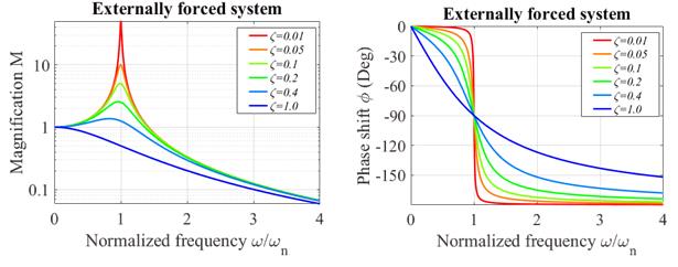
(a)                                                                                (b)

Steady state vibration of a force spring-mass system (a) Magnification (b) phase.

 

 

Solution for Base Excitation

Equation of Motion

$\frac{1}{{\omega }_n^2}\frac{d^{2}x}{d{t}^2}+\frac{2\varsigma }{{\omega }_n}\frac{dx}{dt}+x=K\left(y+\frac{2\varsigma }{{\omega }_n}\frac{dy}{dt}\right)$

with

${\omega }_n=\sqrt{\frac{k}{m}},\varsigma =\frac{\lambda }{2\sqrt{km}},K=1$

Steady State solution

$\begin{array}{c}x(t)=X_0\sin \left(\omega t+\varphi \right)X_0=K{Y}_{0}M(\omega /{\omega }_n,\zeta )\\ M=\frac{{\left\{1+{\left(2\varsigma \omega /{\omega }_n\right)}^2\right\}}^{1/2}}{{\left\{{\left(1-{\omega }^2/{\omega }_n^2\right)}^2+{\left(2\varsigma \omega /{\omega }_n\right)}^2\right\}}^{1/2}}\varphi ={\tan }^{-1}\frac{-2\varsigma {\omega }^3/{\omega }_n^3}{1-(1-4{\varsigma }^2){\omega }^2/{\omega }_n^2}\end{array}$

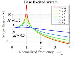
The expressions for $M$ and $\varphi$ are graphed below, as a function of $\omega /{\omega }_n$

 

 

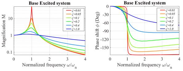
(a)                                                                           (b)

Steady state vibration of a base excited spring$—$mass system (a) Amplitude and (b) phase

 

 

 

 

 

Solution for Rotor Excitation

 

Equation of Motion

$\frac{1}{{\omega }_n^2}\frac{d^{2}x}{d{t}^2}+\frac{2\varsigma }{{\omega }_n}\frac{dx}{dt}+x=-\frac{K}{{\omega }_n^2}\frac{d^{2}y}{d{t}^2}$

with

${\omega }_n=\sqrt{\frac{k}{(m+m_0)}}\varsigma =\frac{\lambda }{2\sqrt{k(m+m_0)}}K=\frac{m_0}{m+m_0}$

Steady state solution

$\begin{array}{c}x(t)=X_0\sin \left(\omega t+\varphi \right)X_0=K{Y}_{0}M(\omega /{\omega }_n,\zeta )\\ M=\frac{{\omega }^2/{\omega }_n^2}{{\left\{{\left(1-{\omega }^2/{\omega }_n^2\right)}^2+{\left(2\varsigma \omega /{\omega }_n\right)}^2\right\}}^{1/2}}\varphi ={\tan }^{-1}\frac{-2\varsigma \omega /{\omega }_n^{}}{1-{\omega }^2/{\omega }_n^2}\end{array}$

 

The expressions for $X_0$ and $\varphi$ are graphed below, as a function of $\omega /{\omega }_n$

 

 

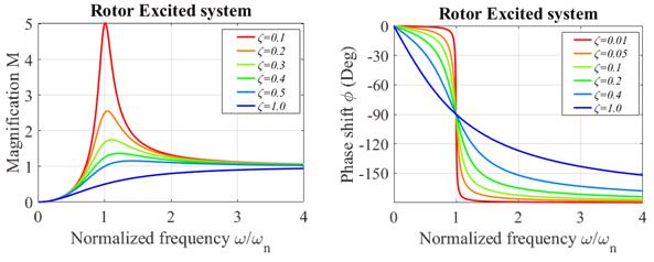
Steady state vibration of a rotor excited spring$—$mass system (a) Amplitude (b) Phase

 

 

5.4.4 Features of the Steady State Response of Spring Mass Systems to Forced Vibrations.

 

 

Now, we will discuss the implications of the results in the preceding section.

 

       The steady state response is always harmonic, and has the same frequency as that of the forcing.

 

To see this mathematically, note that in each case the solution has the form $x(t)=X_0\sin (\omega t+\varphi )$.  Recall that $\omega$ defines the frequency of the force, the frequency of base excitation, or the rotor angular velocity.  Thus, the frequency of vibration is determined by the forcing, not by the properties of the spring-mass system.  This is unlike the free vibration response.

 

You can also check this out using our applet.  To switch off the transient solution, click on the checkbox labeled `show transient’.  Then, try running the applet with different values for k, m and $c$, as well as different forcing frequencies, to see what happens.  As long as you have switched off the transient solution, the response will always be harmonic.

 

       The amplitude of vibration is strongly dependent on the frequency of excitation, and on the properties of the spring$—$mass system.

 

To see this mathematically, note that the solution has the form $x(t)=X_0\sin (\omega t+\varphi )$.  Observe that $X_0$ is the amplitude of vibration, and look at the preceding section to find out how the amplitude of vibration varies with frequency, the natural frequency of the system, the damping factor, and the amplitude of the forcing.  The formulae for $X_0$ are quite complicated, but you will learn a great deal if you are able to sketch graphs of $X_0$ as a function of $\omega /{\omega }_n$ for various values of $\varsigma$. 

 

You can also use our applet to study the influence of forcing frequency, the natural frequency of the system,  and the damping coefficient.  If you plot position-v-time curves, make sure you switch off the transient solution to show clearly the steady state behavior.  Note also that if you click on the `amplitude $–$v- frequency’ radio button just below the graphs, you will see a graph showing the steady state amplitude of vibration as a function of forcing frequency.  The current frequency of excitation is marked as a square dot on the curve (if you don’t see the square dot, it means the frequency of excitation is too high to fit on the scale $–$ if you lower the excitation frequency and press `start’ again you should see the dot appear).  You can change the properties of the spring mass system (or the natural frequency and damping coefficient) and draw new amplitude-v-frequency curves to see how the response of the system has changed. 

 

Try the following tests

 

(i) Keeping the natural frequency fixed (or k and m fixed), plot ampltude-v-frequency graphs for various values of damping coefficient (or the dashpot coefficient).  What happens to the maximum amplitude of vibration as damping is reduced?

 

(ii) Keep the damping coefficient fixed at around 0.1.  Plot graphs of amplitude-v-frequency for various values of the natural frequency of the system.  How does the maximum vibration amplitude change as natural frequency is varied?  What about the frequency at which the maximum occurs?

 

(iii) Keep the dashpot coefficient fixed at a lowish value.  Plot graphs of amplitude-v-frequency for various values of spring stiffness and mass.  Can you reconcile the behavior you observe with the results of test (ii)?

 

(iv) Try changing the type of forcing to base excitation and rotor excitation.  Can you see any differences in the amplitude-v-frequency curves for different types of forcing?

 

(v) Set the damping coefficient to a low value (below 0.1).  Keep the natural frequency fixed.  Run the program for different excitation frequencies.  Watch what the system is doing.  Observe the behavior when the excitation frequency coincides with the natural frequency of the system.  Try this test for each type of excitation.

 

      If the forcing frequency is close to the natural frequency of the system, and the system is lightly damped, huge vibration amplitudes may occur.  This phenomenon is known as resonance. 

 

If you ran the tests in the preceding section, you will have seen the system resonate.  Note that the system resonates at a very similar frequency for each type of forcing.

 

As a general rule, engineers try to avoid resonance like the plague.  Resonance is bad vibrations.  Large amplitude vibrations imply large forces; and large forces cause material failure.  There are exceptions to this rule, of course.  Musical instruments, for example, are supposed to resonate, so as to amplify sound.  Musicians who play string, wind and brass instruments spend years training their lips or bowing arm to excite just the right vibration modes in their instruments to make them sound perfect.  Resonance is a good thing in energy harvesting systems, and many instruments, such as MEMS gyroscopes, and atomic force microscopes, work by measuring how an external stimulus of some sort (rotation, or a surface force) changes the resonant frequency of a system.

 

       There is a phase lag between the forcing and the system response, which depends on the frequency of excitation and the properties of the spring-mass system.

 

The response of the system is $x(t)=X_0\sin (\omega t+\varphi )$.  Expressions for $\varphi$ are given in the preceding section.  Note that the phase lag is always negative. 

 

You can use the applet to examine the physical significance of the phase lag.  Note that you can have the program plot a graph of phase-v-frequency for you, if you wish.

 

It is rather unusual to be particularly interested in the phase of the vibration, so we will not discuss it in detail here.

 

 

5.4.5 Engineering implications of vibration behavior

 

The solutions listed in the preceding sections give us general guidelines for engineering a system to avoid (or create!) vibrations.

 

Preventing a system from vibrating: Suppose that we need to stop a structure or component from vibrating $–$ e.g. to stop a tall building from swaying.   Structures are always deformable to some extent $–$ this is represented qualitatively by the spring in a spring-mass system.  They always have mass $–$ this is represented by the mass of the block.   Finally, the damper represents energy dissipation.  Forces acting on a system generally fluctuate with time.  They probably aren’t perfectly harmonic, but they usually do have a fairly well defined frequency (visualize waves on the ocean, for example, or wind gusts.  Many vibrations are man-made, in which case their frequency is known $–$ for example vehicles traveling on a road tend to induce vibrations with a frequency of about 2Hz, corresponding to the bounce of the car on its suspension).

So how do we stop the system from vibrating?   We know that its motion is given by

$\begin{array}{c}x(t)=X_0\sin \left(\omega t+\varphi \right)\\ X_0=\frac{K{F}_0}{{\left\{{\left(1-{\omega }^2/{\omega }_n^2\right)}^2+{\left(2\varsigma \omega /{\omega }_n\right)}^2\right\}}^{1/2}}\\ \varphi ={\tan }^{-1}\frac{-2\varsigma \omega /{\omega }_n}{1-{\omega }^2/{\omega }_n^2}\end{array}$

${\omega }_n=\sqrt{\frac{k}{m}},\varsigma =\frac{c}{2\sqrt{km}},K=\frac{1}{k}$

To minimize vibrations, we must design the system to make the vibration amplitude $X_0$ as small as possible.  The formula for $X_0$ is a bit scary, which is why we plot graphs of the solution.  The graphs show that we will observe vibrations with large amplitudes if (i) The frequency  $\omega /{\omega }_n$ is close to 1; and (ii) the damping $\zeta$ is small.  At first sight, it looks like we could minimize vibrations by making $\omega /{\omega }_n$ very large.  This is true in principle, and can be done in some designs, e.g. if the force acts on a very localized area of the structure, and will only excite a single vibration mode.  For most systems, this approach will not work, however.  This is because real components generally have a very large number of natural frequencies of vibration, corresponding to different vibration modes.   We could design the system so that $\omega /{\omega }_n$ is large for the mode with the lowest frequency $–$ and perhaps some others $–$ but there will always be other modes with higher frequencies, which will have smaller values of  $\omega /{\omega }_n$ .  There is a risk that one of these will be close to resonance.  Consequently, we generally design the system so that $\omega /{\omega }_n<<1$ for the mode with the lowest natural frequency.  In fact, design codes usually specify the minimum allowable value of  $\omega /{\omega }_n$ for vibration critical components.  This will guarantee that $\omega /{\omega }_n<<1$ for all modes, and hence the vibration amplitude $X_0\to K{F}_0=F_0/k$.  This tells us that the best approach to avoid vibrations is to make the structure as stiff as possible.  This will make the natural frequency large, and will also make $F_0/k$ small.

 

Designing a suspension or vibration isolation system.  Suspensions, and vibration isolation systems, are examples of base excited systems.  In this case, the system really consists of a mass (the vehicle, or the isolation table) on a spring (the shock absorber or vibration isolation pad).  We expect that the base will vibrate with some characteristic frequency $\omega$. Our goal is to design the system to minimize the vibration of the mass.

 

Our vibration solution predicts that the mass vibrates with displacement

$\begin{array}{c}x(t)=X_0\sin \left(\omega t+\varphi \right)\\ X_0=\frac{K{Y}_0{\left\{1+{\left(2\varsigma \omega /{\omega }_n\right)}^2\right\}}^{1/2}}{{\left\{{\left(1-{\omega }^2/{\omega }_n^2\right)}^2+{\left(2\varsigma \omega /{\omega }_n\right)}^2\right\}}^{1/2}}\\ \varphi ={\tan }^{-1}\frac{-2\varsigma {\omega }^3/{\omega }_n^3}{1-(1-4{\varsigma }^2){\omega }^2/{\omega }_n^2}\end{array}$

${\omega }_n=\sqrt{\frac{k}{m}},\varsigma =\frac{c}{2\sqrt{km}},K=1$

Again, the graph is helpful to understand how the vibration amplitude $X_0$ varies with system parameters.

 

Clearly, we can minimize the vibration amplitude of the mass by making $\omega /{\omega }_n>>1$.   We can do this by making the spring stiffness as small as possible (use a soft spring), and making the mass large.  It also helps to make the damping $\zeta$ small.  This is counter-intuitive $–$ people often think that the energy dissipated by the shock absorbers in their suspensions that makes them work.   There are some disadvantages to making the damping too small, however.  For one thing, if the system is lightly damped, and is disturbed somehow, the subsequent transient vibrations will take a very long time to die out.   In addition, there is always a risk that the frequency of base excitation is lower than we expect $–$ if the system is lightly damped, a potentially damaging resonance may occur.  

 

Suspension design involves a bit more than simply minimizing the vibration of the mass, of course $–$ the car will handle poorly if the wheels begin to leave the ground.  A very soft suspension generally has poor handling, so the engineers must trade off handling against vibration isolation.

 

 

 

 

5.4.6 Using Forced Vibration Response to Measure Properties of a System.

 

We often measure the natural frequency and damping coefficient for a mode of vibration in a structure or component, by measuring the forced vibration response of the system.

 

Here is how this is done.  We find some way to apply a harmonic excitation to the system (base excitation might work; or you can apply a force using some kind of actuator, or you could deliberately mount an unbalanced rotor on the system).

Then, we mount accelerometers on our system, and use them to measure the displacement of the structure, at the point where it is being excited, as a function of frequency.

 

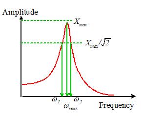
We then plot a graph, which usually looks something like the picture on the right. We read off the maximum response $X_{\max }$, and draw a horizontal line at amplitude $X_{\max }/\sqrt{2}$.  Finally, we measure the frequencies ${\omega }_1$, ${\omega }_2$ and ${\omega }_{\max }$ as shown in the picture.

 

We define the bandwidth of the response $\Delta \omega$ as

$\Delta \omega ={\omega }_2-{\omega }_1$

Like the logarithmic decrement, the bandwidth of the forced harmonic response is a measure of the damping in a system.

 

It turns out that we can estimate the natural frequency of the system and its damping coefficient using the following formulae

$\varsigma \approx \frac{\Delta \omega }{2{\omega }_{\max }}{\omega }_n\approx {\omega }_{\max }$

The formulae are accurate for small $\varsigma$ - say $\varsigma <0.2$.

 

To understand the origin of these formulae, recall that the amplitude of vibration due to external forcing is given by

$X_0=\frac{K{F}_0}{\sqrt{{\left(1-{\omega }^2/{\omega }_n^2\right)}^2+{\left(2\varsigma \omega /{\omega }_n\right)}^2}}$

We can find the frequency at which the amplitude is a maximum by differentiating with respect to $\omega$, setting the derivative equal to zero and solving the resulting equation for frequency.  It turns out that the maximum amplitude occurs at a frequency

${\omega }_{\max }={\omega }_n\sqrt{1-2{\varsigma }^2}$

For small $\varsigma$, we see that

${\omega }_{\max }\approx {\omega }_n$

 

 

Next, to get an expression relating the bandwidth $\Delta \omega$ to $\varsigma$, we first calculate the frequencies ${\omega }_1$ and ${\omega }_2$.  Note that the maximum amplitude of vibration can be calculated by setting $\omega ={\omega }_{\max }$, which gives

$X_{\max }=\frac{K{F}_0}{2\varsigma \sqrt{1-{\varsigma }^2}}$

Now, at the two frequencies of interest, we know $X_0=X_{\max }/\sqrt{2}$, so that ${\omega }_1$ and ${\omega }_2$ must be solutions of the equation

$\frac{K{F}_0}{2\varsigma \sqrt{1-{\varsigma }^2}}\frac{1}{\sqrt{2}}=\frac{K{F}_0}{\sqrt{{\left(1-{\omega }^2/{\omega }_n^2\right)}^2+{\left(2\varsigma \omega {\omega }_n\right)}^2}}$

Rearrange this equation to see that

${\omega }^4-2{\omega }^2{\omega }_n^2(1-2{\varsigma }^2)+{\omega }_n^4-8{\varsigma }^2{\omega }_n^4(1-{\varsigma }^2)=0$

This is a quadratic equation for ${\omega }^2$ and has solutions

$\begin{array}{l}{\omega }_1^{}={\left\{{\omega }_n^2(1-2{\varsigma }^2)-2{\omega }_n^2\varsigma \sqrt{1-{\varsigma }^2}\right\}}^{1/2}\\ {\omega }_2^{}={\left\{{\omega }_n^2(1-2{\varsigma }^2)+2{\omega }_n^2\varsigma \sqrt{1-{\varsigma }^2}\right\}}^{1/2}\end{array}$

Expand both expressions in a Taylor series about $\varsigma =0$ to see that

$\begin{array}{l}{\omega }_1\approx {\omega }_n(1-\varsigma )\\ {\omega }_2\approx {\omega }_n(1+\varsigma )\end{array}$

so, finally, we confirm that

$\Delta \omega ={\omega }_2-{\omega }_1=2\varsigma {\omega }_n$

 

 

5.4.7 Example Problems in Forced Vibrations

 

Example 1: A structure is idealized as a damped spring$—$mass system with stiffness 10 kN/m; mass 2Mg; and dashpot coefficient 2 kNs/m.  It is subjected to a harmonic force of amplitude 500N at frequency 0.5Hz.  Calculate the steady state amplitude of vibration.

 

Start by calculating the properties of the system:

${\omega }_n=\sqrt{\frac{k}{m}}=2.23\text{ rad/s}\varsigma =\frac{c}{2\sqrt{km}}=0.224K=\frac{1}{k}=\frac{1}{10000}\text{ m/N}$

Now, the list of solutions to forced vibration problems gives

$\begin{array}{c}x(t)=X_0\sin \left(\omega t+\varphi \right)\\ X_0=\frac{K{F}_0}{{\left\{{\left(1-{\omega }^2/{\omega }_n^2\right)}^2+{\left(2\varsigma \omega /{\omega }_n\right)}^2\right\}}^{1/2}}\varphi ={\tan }^{-1}\frac{-2\varsigma \omega /{\omega }_n}{1-{\omega }^2/{\omega }_n^2}\end{array}$

For the present problem:

$\omega =0.5\times 2\pi \text{rad/s}\Rightarrow \omega \text{/}{\omega }_{\text{n}}=\pi /2.23=1.41$

Substituting numbers into the expression for the vibration amplitude shows that

$X_0=43\text{mm}$

 

 

Example 2: A car and its suspension system are idealized as a damped spring$—$mass system, with natural frequency 0.5Hz and damping coefficient 0.2.  Suppose the car drives at speed V over a road with sinusoidal roughness.  Assume the roughness wavelength is 10m, and its amplitude is 20cm.  At what speed does the maximum amplitude of vibration occur, and what is the corresponding vibration amplitude?

 

Let s denote the distance traveled by the car, and let L denote the wavelength of the roughness and H the roughness amplitude.  Then, the height of the wheel above the mean road height may be expressed as

$y=H\sin \left(\frac{2\pi s}{L}\right)$

Noting that $s=Vt$, we have that

$y(t)=H\sin \left(\frac{2\pi V}{L}t\right)$

i.e., the wheel oscillates vertically with harmonic motion, at frequency $\omega =2\pi V/L$.

 

Now, the suspension has been idealized as a spring$—$mass system subjected to base excitation.  The steady state vibration is

$\begin{array}{c}x(t)=X_0\sin \left(\omega t+\varphi \right)X_0=K{Y}_{0}M\\ M=\frac{{\left\{1+{\left(2\varsigma \omega /{\omega }_n\right)}^2\right\}}^{1/2}}{{\left\{{\left(1-{\omega }^2/{\omega }_n^2\right)}^2+{\left(2\varsigma \omega /{\omega }_n\right)}^2\right\}}^{1/2}}\varphi ={\tan }^{-1}\frac{-2\varsigma {\omega }^3/{\omega }_n^3}{1-(1-4{\varsigma }^2){\omega }^2/{\omega }_n^2}\end{array}$

For light damping, the maximum amplitude of vibration occurs at around the natural frequency.  Therefore, the critical speed follows from

$\begin{array}{l}\omega =\frac{2\pi V}{L}={\omega }_n\\ \Rightarrow V={\omega }_{n}L/2\pi =5\text{m/s=18 km/hr}\end{array}$

Note that K=1 for base excitation, so that the amplitude of vibration at $\omega /{\omega }_n=1$ is approximately

$X_0\approx \frac{Y_0}{2\varsigma }=20/0.4=50\text{cm}$

Note that at this speed, the suspension system is making the vibration worse.  The amplitude of the car’s vibration is greater than the roughness of the road.  Suspensions work best if they are excited at frequencies well above their resonant frequencies. 

 

 

Example 3: The suspension system discussed in the preceding problem has the following specifications.  For the roadway described in the preceding section, the amplitude of vibration may not exceed 35cm at any speed.  At 55 miles per hour, the amplitude of vibration must be less than 10cm.  The car weighs 3000lb.  Select values for the spring stiffness and the dashpot coefficient.

                              

We must first determine values for $\zeta$ and ${\omega }_n$ that will satisfy the design specifications. To this end:

(i)                 The specification requires that

$\frac{X_0}{Y_0}<\frac{35}{20}=1.75$

for any value of $\omega$ (remember $\omega =2\pi V/L$ ).  Recall that $X_0=K{Y}_{0}M(\omega /{\omega }_n,\zeta )$ and that K=1 for a base excited spring$—$mass system. This tells us that the magnification $M=X_0/Y_0$ has to be below 1.75 for any frequency. The graph shows that if $\varsigma >0.4$, the magnification never exceeds 1.75.  We also see that smaller values of $\zeta$ make the suspension more effective (M is smaller) at high frequencies.   So $\varsigma =0.4$ is a good choice.

 

If you prefer not to use the graph, you can use the approximation $M_{\max }\approx 1/(2\zeta )$ which suggests that $\zeta >1/(2\times 1.75)$ which gives $\zeta \approx 0.3$ - but the approximation is not very accurate for such large values of $\zeta$ (to get a better estimate you’d have to maximize the formula for magnification with respect to $\omega$ but that’s very messy).

 

(ii)               Now, the frequency of base excitation at 55mph is

$\omega =\frac{2\pi V}{L}=\frac{2\pi \times 0.447\times 55}{10}=15.45\text{ rad/s}$

We must choose system parameters so that, at this excitation frequency, $X_0/Y_0<10/20=1/2$.

This tells us that M must be less than $\mathrm{½}$ when $\omega$ is 15.45 rad/s or greater.  We already know that $\zeta =0.4$, and following the curve for this value of $\zeta$ we see that M<1/2 if  $\omega /{\omega }_n>2$. Therefore, we must pick ${\omega }_n<\omega /2=7.7\text{ rad/s}$.

 

Again, if you prefer not to use the graph, you can also solve

$M=\frac{{\left\{1+{\left(2\varsigma \omega /{\omega }_n\right)}^2\right\}}^{1/2}}{{\left\{{\left(1-{\omega }^2/{\omega }_n^2\right)}^2+{\left(2\varsigma \omega /{\omega }_n\right)}^2\right\}}^{1/2}}<\frac{1}{2}$

for $\omega /{\omega }_n$ , but this is a pain, and the graph is accurate enough for a design estimate.

Finally, we can compute properties of the system.  We have that

${\omega }_n=\sqrt{\frac{k}{m}}\Rightarrow 7.7=\sqrt{\frac{k}{0.44\times 3000}}\Rightarrow k=78\text{ kN/m}$

Similarly

$\varsigma =\frac{\lambda }{2\sqrt{mk}}\Rightarrow \lambda =2\times 0.4\times \sqrt{78000\times .44\times 3000}=8\text{kNs/m}$

5.5 Solving differential equations for vibrating systems

 

Our goal in this course is to understand what the solutions to differential equations tell us about engineering problems we might need to solve.   But if you have time on your hands, you might be interested in learning how to solve the differential equations. It’s fairly straightforward, if a little tedious algebraically.  You will learn this material in future courses (applied math, and several more advanced engineering courses) whether you want to or not…  

 

Review of complex numbers

It’s easiest to solve linear ODEs using complex variables.   The following definitions and results are particularly useful:

 Define $i=\sqrt{-1}$ 

 Any complex number z can be split into imaginary and real parts as

$z=a+ib$

where a and b are two real numbers.

 Define the complex conjugate as $\overline{z}=a-ib$ 

 It follows that  $a=(z+\overline{z})/2b=-i(z-\overline{z})/2$ 

 The exponential of an imaginary number (Euler’s formula) is

$e^{i\theta }=\cos \theta +i\sin \theta$

You can prove this by taking the Taylor expansion of both sides of the formula

 Euler’s formula enables us to write any complex number in polar form

$\begin{array}{l}a+ib=\rho e^{i\theta }\rho =\sqrt{a^2+b^2}\theta ={\tan }^{-1}(b/a)\\ a=\rho \cos \theta b=\rho \sin \theta \end{array}$

 Euler’s formula also allows us to represent trig functions as complex exponentials

$\cos \theta =(e^{i\theta }+e^{-i\theta })/2\sin \theta =-i(e^{i\theta }-e^{-i\theta })/2$

 Note that

$\frac{d{e}^{i\omega t}}{dt}=i\omega e^{i\omega t}\frac{d^2{e}^{i\omega t}}{d{t}^2}=-{\omega }^2{e}^{i\omega t}$

 

Solution to the equation of motion for an undamped harmonic oscillator

Solve $\frac{1}{{\omega }_n^2}\frac{d^{2}x}{d{t}^2}+x=C$ with initial conditions $x=x_{0}dx/dt=v_{0}t=0$ 

Guess a solution of the form $x=C+A{e}^{\lambda t}$ where A and $\lambda$ are two complex numbers to be determined  (this may seem a cheat, but actually there are only two ways to do an integral (1) guess a solution, differentiate it, and see if the answer is correct; and (2) rearrange the integral into another form with a known solution.   We know an exponential is a good guess for x because when an exponential is differentiated it stays an exponential).   Substitute this into our ODE

$\frac{{\lambda }^2}{{\omega }_n^2}A{e}^{\lambda t}+A{e}^{\lambda t}=0$

We can satisfy this for any A by choosing ${\lambda }^2/{\omega }_n^2=-1\Rightarrow \lambda =\pm \sqrt{-1}{\omega }_n=\pm i{\omega }_n$ .   This gives us two families of solutions to the equations, one with $x=C+A\exp (i{\omega }_{n}t)$ and another with $x=A\exp (-i{\omega }_{n}t)$.  The most general solution is the sum of these, with different coefficients

$x=C+A_1{e}^{i{\omega }_{n}t}+A_2{e}^{-i{\omega }_{n}t}$

We need to find $A_1,A_2$: we can do this by substituting t=0 into x and using the given values of x at t=0

$\begin{array}{l}x(0)=A_1+A_2+C=x_0\Rightarrow A_1+A_2=x_0-C\\ {\frac{dx}{dt}|}_{t=0}=i{\omega }_n(A_1-A_2)=v_0\Rightarrow A_1-A_2=-i{v}_0/{\omega }_n\end{array}$

Add and subtract these two equations to see that

$A_1=\frac{1}{2}\left((x_0-C)-i\frac{v_0}{{\omega }_n}\right)A_2=\frac{1}{2}\left((x_0-C)+i\frac{v_0}{{\omega }_n}\right)$

We can use Euler’s formula to re-write this as

$\begin{array}{l}{A}_1=-\frac{i}{2}{X}_0{e}^{i\varphi }{A}_2=\frac{i}{2}{X}_0{e}^{-i\varphi }\\ X_0=\sqrt{{\left(x_0-C\right)}^2+v_0^2/{\omega }_n^2}\sin \varphi =\frac{x_0-C}{\sqrt{{\left(x_0-C\right)}^2+v_0^2/{\omega }_n^2}}\cos \varphi =\frac{v_0/{\omega }_n}{\sqrt{{\left(x_0-C\right)}^2+v_0^2/{\omega }_n^2}}\end{array}$

(to see this just substitute $X_0,\varphi$ into the formulas and use Euler’s formula to show $A_1,A_2$  are correct).  Finally substitute $A_1,A_2$ into the general solution for x to see that

$\begin{array}{l}x=C-\frac{i}{2}{X}_0{e}^{i\varphi }{e}^{i{\omega }_{n}t}+\frac{i}{2}{X}_0{e}^{-i\varphi }{e}^{-i{\omega }_{n}t}=C-\frac{i}{2}{X}_0\left(e^{i({\omega }_{n}t+\varphi )}-e^{-i({\omega }_{n}t+\varphi )}\right)\\ =C+X_0\sin ({\omega }_{n}t+\varphi )\end{array}$

This agrees with the answer on the formula sheet.

 

 

Solution to the equation of motion for a free damped system

 

Solve $\frac{1}{{\omega }_n^2}\frac{d^{2}x}{d{t}^2}+\frac{2\varsigma }{{\omega }_n}\frac{dx}{dt}+x=C$ with initial conditions $x=x_{0}dx/dt=v_{0}t=0$

 

As before we guess a solution $x=C+A{e}^{\lambda t}$ where A and $\lambda$ are two complex numbers to be determined.  Substituting into the equation:

$\left(\frac{{\lambda }^2}{{\omega }_n^2}+\frac{2\varsigma \lambda }{{\omega }_n}+1\right)A{e}^{\lambda t}=0$

This gives a quadratic equation for $\lambda$ (it is called the ‘characteristic equation’ for the differential equation).  It has solutions

$\lambda =-\zeta {\omega }_n\mp {\omega }_n\sqrt{{\zeta }^2-1}$

Depending on the value of $\zeta$ we find

·         $\zeta >1$  (overdamped) $–$ two real values of $\lambda$ $\lambda =-\zeta {\omega }_n\pm {\omega }_d$ 

·         $\zeta =1$  (critical damping): $\lambda =-{\omega }_n$ 

·         $\zeta <1$ (underdamped) $–$ two complex values of $\lambda$ $\lambda =-\zeta {\omega }_n\pm i{\omega }_d$

where we have defined ${\omega }_d={\omega }_n\sqrt{\left|{\zeta }^2-1\right|}$  To write the answers in terms of real valued functions we need to treat these cases separately.

 

Overdamped solution: We have that

$x=C+A_1{e}^{(-\zeta {\omega }_n+{\omega }_d)t}+A_2{e}^{(-\zeta {\omega }_n-{\omega }_d)t}$

We can use the initial conditions to determine $A_1,A_2$ :

$\begin{array}{l}x(0)=C+A_1+A_2=x_0\\ {\frac{dx}{dt}|}_{t=0}=A_1({\omega }_d-\zeta {\omega }_n)-A_1({\omega }_d+\zeta {\omega }_n)=v_0\\ \Rightarrow A_1=\frac{v_0+(\varsigma {\omega }_n+{\omega }_d)(x_0-C)}{2{\omega }_d}{A}_2=-\frac{v_0+(\varsigma {\omega }_n-{\omega }_d)(x_0-C)}{2{\omega }_d}\end{array}$

Hence

$x(t)=C+\exp (-\varsigma {\omega }_{n}t)\left\{\frac{v_0+(\varsigma {\omega }_n+{\omega }_d)(x_0-C)}{2{\omega }_d}\exp ({\omega }_{d}t)-\frac{v_0+(\varsigma {\omega }_n-{\omega }_d)(x_0-C)}{2{\omega }_d}\exp (-{\omega }_{d}t)\right\}$

 

 

 

Critically damped solution: our guess for the critically damped solution gives only $x=C+A_1{e}^{-\zeta {\omega }_{n}t}$ which cannot satisfy the initial conditions on both x and dx/dt, so the solution is incomplete.   We have to look around for another solution $–$ it turns out that

$x=C+A_1{e}^{-{\omega }_{n}t}+A_{2}t{e}^{-{\omega }_{n}t}$

will also satisfy the differential equation (this is a standard trick in situations where the characteristic equation has repeated roots).   We can solve for $A_1,A_2$ using the initial conditions:

$\begin{array}{l}x(0)=C+A_1=x_0\\ {\frac{dx}{dt}|}_{t=0}=-{\omega }_n{A}_1+A_2=v_0\end{array}$

It follows that $A_1=x_0-C{A}_2=v_0+{\omega }_n(x_0-C)$ so the solution is

$x(t)=C+\left\{(x_0-C)+\left[v_0+{\omega }_n(x_0-C)\right]t\right\}\exp (-{\omega }_{n}t)$

 

Underdamped solution: For this case

$x=C+A_1{e}^{(-\zeta {\omega }_n+i{\omega }_d)t}+A_2{e}^{(-\zeta {\omega }_n-i{\omega }_d)t}$

We can use the initial conditions to determine $A_1,A_2$ (which are now complex):

$\begin{array}{l}x(0)=C+A_1+A_2=x_0\\ {\frac{dx}{dt}|}_{t=0}=A_1(i{\omega }_d-\zeta {\omega }_n)-A_1(i{\omega }_d+\zeta {\omega }_n)=v_0\\ \Rightarrow A_1=-i\frac{v_0+(\varsigma {\omega }_n+i{\omega }_d)(x_0-C)}{2{\omega }_d}{A}_2=i\frac{v_0+(\varsigma {\omega }_n-i{\omega }_d)(x_0-C)}{2{\omega }_d}\end{array}$

We can substitute this back into the solution and re-arrange the result

$x(t)=C+\exp (-\varsigma {\omega }_{n}t)\left\{(x_0-C)\frac{1}{2}\left(e^{i{\omega }_{d}t}+e^{-i{\omega }_{d}t}\right)-\frac{v_0+\varsigma {\omega }_n(x_0-C)}{\omega {}_d}\frac{i}{2}\left(e^{i{\omega }_{d}t}-e^{-i{\omega }_{d}t}\right)\right\}$

Finally we recognize the combinations of complex exponentials as trig functions, giving

$x(t)=C+\exp (-\varsigma {\omega }_{n}t)\left\{(x_0-C)\cos {\omega }_{d}t+\frac{v_0+\varsigma {\omega }_n(x_0-C)}{\omega {}_d}\sin {\omega }_{d}t\right\}$

 

 

 

Solution to the equation of motion for a system subjected to harmonic external force

Solve $\frac{1}{{\omega }_n^2}\frac{d^{2}x}{d{t}^2}+\frac{2\varsigma }{{\omega }_n}\frac{dx}{dt}+x=C+K{F}_0\sin \omega t$ with initial conditions $x=x_{0}dx/dt=v_{0}t=0$

It is helpful to replace the trig function with its equivalent representation in terms of complex exponentials

$\frac{1}{{\omega }_n^2}\frac{d^{2}x}{d{t}^2}+\frac{2\varsigma }{{\omega }_n}\frac{dx}{dt}+x=C-K{F}_0\frac{i}{2}\left(e^{i\omega t}-e^{-i\omega t}\right)$

We guess a solution of the form

$\begin{array}{l}x(t)=x_p(t)+x_h(t)\\ x_p(t)=-\frac{i}{2}\left(B_1{e}^{i\omega t}-B_2{e}^{-i\omega t}\right)x_h=C+A{e}^{\lambda t}\end{array}$

where  $B_1,B_2,A,\lambda$ are complex numbers to be determined.   Substituting into the ODE:

$\left(\frac{{\lambda }^2}{{\omega }_n^2}+\frac{2\varsigma \lambda }{{\omega }_n}+1\right)A{e}^{\lambda t}-\frac{i}{2}\left(\left(1-\frac{{\omega }^2}{{\omega }_n^2}+\frac{2\varsigma \omega }{{\omega }_n}i\right)B_1{e}^{i\omega t}-\left(1-\frac{{\omega }^2}{{\omega }_n^2}-\frac{2\varsigma \omega }{{\omega }_n}i\right)B_2{e}^{-i\omega t}\right)=-K{F}_0\frac{i}{2}\left(e^{i\omega t}-e^{-i\omega t}\right)$

 We can satisfy this by setting

$B_1\left(1-\frac{{\omega }^2}{{\omega }_n^2}+\frac{2\varsigma \omega }{{\omega }_n}i\right)=K{F}_0{B}_2\left(1-\frac{{\omega }^2}{{\omega }_n^2}-\frac{2\varsigma \omega }{{\omega }_n}i\right)=K{F}_0\left(\frac{{\lambda }^2}{{\omega }_n^2}+\frac{2\varsigma \lambda }{{\omega }_n}+1\right)=0$

The first two equations show that

$\begin{array}{l}{B}_1=K{F}_0{\left(1-\frac{{\omega }^2}{{\omega }_n^2}+\frac{2\varsigma \omega }{{\omega }_n}i\right)}^{-1}=K{F}_{0}M(\omega /{\omega }_n,\zeta )e^{i\varphi }\\ B_2=K{F}_0{\left(1-\frac{{\omega }^2}{{\omega }_n^2}-\frac{2\varsigma \omega }{{\omega }_n}i\right)}^{-1}=K{F}_{0}M(\omega /{\omega }_n,\zeta )e^{-i\varphi }\\ M(\omega /{\omega }_n,\zeta )=\frac{1}{\sqrt{{\left(1-\frac{{\omega }^2}{{\omega }_n^2}\right)}^2+{\left(\frac{2\varsigma \omega }{{\omega }_n}\right)}^2}}\varphi ={\tan }^{-1}\frac{-2\zeta \omega /{\omega }_n}{(1-{\omega }^2/{\omega }_n^2)}\end{array}$

(we introduced M and $\varphi$ to re-write $B_1,B_2$ in polar form).  Finally substitute back for $B_1,B_2$ into the guess for $x_p(t)$ and simplify the solution to see that

$x_p(t)=-\frac{i}{2}K{F}_{0}M(\omega /{\omega }_n,\zeta )\left(e^{i(\omega t+\varphi )}-e^{-i(\omega t+\varphi )}\right)=K{F}_{0}M(\omega /{\omega }_n,\zeta )\sin (\omega t+\varphi )$

Finally, we must determine $x_h(t)$ .  By construction, our guess for $x_h(t)$ satisfies

$\begin{array}{l}\frac{1}{{\omega }_n^2}\frac{d^2{x}_h}{d{t}^2}+\frac{2\varsigma }{{\omega }_n}\frac{d{x}_h}{dt}+x_h=C\\ x_h(0)=x_0-x_p(0)=x_0-X_0\sin \varphi \\ {\frac{d{x}_h}{dt}|}_{t=0}=v_0-{\frac{d{x}_p}{dt}|}_{t=0}=v_0-X_0\omega \cos \varphi \end{array}$

This is identical to the differential equation for a damped free vibrating system (but with modified initial conditions), and we can just write down the solution from the preceding section.

Short-cut for calculating steady-state solutions for forced vibrating systems

 

For example, consider the base excited system

$\frac{1}{{\omega }_n^2}\frac{d^{2}x}{d{t}^2}+\frac{2\varsigma }{{\omega }_n}\frac{dx}{dt}+x=C+K\left(1+\frac{2\varsigma }{{\omega }_n}\frac{d}{dt}\right)Y_0\sin \omega t$

We anticipate that the steady-state solution will have the form

$x_p(t)=X_0\sin (\omega t+\varphi )X_0=K{Y}_{0}M(\omega /{\omega }_n,\zeta )$

so we only need to determine the magnification $M$ and the phase $\varphi$ .   We can do this quickly by

(i)     Replacing the harmonic function $Y_0\sin \omega t$ by a complex exponential $Y_0{e}^{i\omega t}$ 

(ii)   Substituting $x=C+K{Y}_{0}M{e}^{i\varphi }{e}^{i\omega t}$ into the solution

This gives

$K{Y}_{0}M{e}^{i\varphi }\left(1-\frac{{\omega }^2}{{\omega }_n^2}+i\frac{2\varsigma \omega }{{\omega }_n}\right)e^{i\omega t}=K\left(1+i\frac{2\varsigma \omega }{{\omega }_n}\right)Y_0{e}^{i\omega t}$

Hence

$M{e}^{i\varphi }=\frac{\left(1+i\frac{2\varsigma \omega }{{\omega }_n}\right)}{\left(1-\frac{{\omega }^2}{{\omega }_n^2}+i\frac{2\varsigma \omega }{{\omega }_n}\right)}$

Finally, write the complex numbers on the right hand side in polar form and read off M and $\varphi$ 

$M=\frac{\sqrt{1+{\left(\frac{2\varsigma \omega }{{\omega }_n}\right)}^2}}{\sqrt{{\left(1-\frac{{\omega }^2}{{\omega }_n^2}\right)}^2+{\left(\frac{2\varsigma \omega }{{\omega }_n}\right)}^2}}\varphi ={\tan }^{-1}\frac{2\varsigma \omega }{{\omega }_n}-{\tan }^{-1}\frac{\frac{2\varsigma \omega }{{\omega }_n}}{\left(1-\frac{{\omega }^2}{{\omega }_n^2}\right)}$

Similarly, to find the magnification and phase for the rotor-excited system, which has differential equation

$\frac{1}{{\omega }_n^2}\frac{d^{2}x}{d{t}^2}+\frac{2\varsigma }{{\omega }_n}\frac{dx}{dt}+x=C-\frac{K}{{\omega }_n^2}\frac{d^{2}y}{d{t}^2}$

we make the substitutions (i) and (ii) above and simplify the result to see that:

$M{e}^{i\varphi }=\frac{{\omega }^2/{\omega }_n^2}{\left(1-\frac{{\omega }^2}{{\omega }_n^2}+i\frac{2\varsigma \omega }{{\omega }_n}\right)}$

Re-write the right hand side in polar form

$M=\frac{{\omega }^2/{\omega }_n^2}{\sqrt{{\left(1-\frac{{\omega }^2}{{\omega }_n^2}\right)}^2+{\left(\frac{2\varsigma \omega }{{\omega }_n}\right)}^2}}\varphi ={\tan }^{-1}\frac{-2\varsigma \omega /{\omega }_n}{\left(1-\frac{{\omega }^2}{{\omega }_n^2}\right)}$

You will learn even faster tricks for solving differential equations in circuits next semester, and perhaps in more advanced level linear systems and control theory courses.   In fact, the pros know tricks that avoid writing down the differential equation altogether $–$ they can just go straight to the solution!   If you want to develop these superpowers, stick with engineering, and keep writing those generous tuition checks!

 

5.6 Introduction to vibration of systems with many degrees of freedom

 

The simple 1DOF systems analyzed in the preceding section are very helpful to develop a feel for the general characteristics of vibrating systems.   They are too simple to approximate most real systems, however.   Real systems have more than just one degree of freedom.   Real systems are also very rarely linear.   You may be feeling cheated $–$ are the simple idealizations that you get to see in intro courses really any use?   It turns out that they are, but you can only really be convinced of this if you know how to analyze more realistic problems, and see that they often behave just like the simple idealizations. 

 

The motion of systems with many degrees of freedom, or nonlinear systems, cannot usually be described using simple formulas. Even when they can, the formulas are so long and complicated that you need a computer to evaluate them.  For this reason, introductory courses typically avoid these topics.  However, if you are willing to use a computer, analyzing the motion of these complex systems is actually quite straightforward $–$ in fact, often easier than using the nasty formulas we derived for 1DOF systems. 

 

This section of the notes is intended mostly for advanced students, who may be insulted by simplified models.  If you are feeling insulted, read on…

 

5.6.1 Equations of motion for undamped linear systems with many degrees of freedom.

 

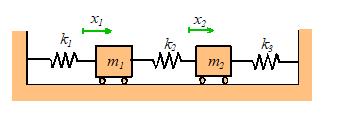We always express the equations of motion for a system with many degrees of freedom in a standard form.  The two degree of freedom system shown in the picture can be used as an example.  We won’t go through the calculation in detail here (you should be able to derive it for yourself $–$ draw a FBD, use Newton’s law and all that tedious stuff), but here is the final answer:

 

$\begin{array}{l}{m}_1\frac{d^2{x}_1}{d{t}^2}+\left(k_1+k_2\right)x_1-k_2{x}_2=0\\ m_2\frac{d^2{x}_2}{d{t}^2}-k_2{x}_1+(k_2+k_3)x_2=0\end{array}$

To solve vibration problems, we always write the equations of motion in matrix form.  For an undamped system, the matrix equation of motion always looks like this

$M\frac{d^{2}x}{d{t}^2}+Kx=0$

where x is a vector of the variables describing the motion,  M is called the ‘mass matrix’ and K is called the ‘Stiffness matrix’ for the system.  For the two spring-mass example, the equation of motion can be written in matrix form as

$\left[\begin{array}{cc}{m}_1& 0\\ 0& m_2\end{array}\right]\frac{d^2}{d{t}^2}\left[\begin{array}{c}{x}_1\\ x_2\end{array}\right]+\left[\begin{array}{cc}{k}_1+k_2& -k_2\\ -k_2& k_2+k_3\end{array}\right]\left[\begin{array}{c}{x}_1\\ x_2\end{array}\right]=\left[\begin{array}{c}0\\ 0\end{array}\right]$

For a system with two masses (or more generally, two degrees of freedom), M and K are 2x2 matrices.  For a system with n degrees of freedom, they are nxn matrices.

 

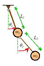The spring-mass system is linear.  A nonlinear system has more complicated equations of motion, but these can always be arranged into the standard matrix form by assuming that the displacement of the system is small, and linearizing the equation of motion.   For example, the full nonlinear equations of motion for the double pendulum shown in the figure are

$\begin{array}{l}(m_1+m_2)L_1{\ddot{\theta }}_1+m_2{L}_2{\dot{\theta }}_2^2\sin ({\theta }_1-{\theta }_2)+m_2{L}_2{\ddot{\theta }}_2\cos ({\theta }_1-{\theta }_2)+(m_1+m_2)g\sin {\theta }_1=0\\ m_2{L}_2{\ddot{\theta }}_2+m_2{L}_1{\ddot{\theta }}_1\cos ({\theta }_1-{\theta }_2)-m_2{L}_1{\dot{\theta }}_1^2\sin ({\theta }_1-{\theta }_2)+m_{2}g\sin {\theta }_2=0\end{array}$

Here, a single dot over a variable represents a time derivative, and a double dot represents a second time derivative (i.e. acceleration). These equations look horrible (and indeed they are $–$ the motion of a double pendulum can even be chaotic), but if we assume that if ${\theta }_1$, ${\theta }_2$, and their time derivatives are all small, so that terms involving squares, or products, of these variables can all be neglected, that and recall that $\cos (x)\approx 1$ and $\sin (x)\approx x$ for small x, the equations simplify to

$\begin{array}{l}(m_1+m_2)L_1{\ddot{\theta }}_1+m_2{L}_2{\ddot{\theta }}_2+(m_1+m_2)g{\theta }_1=0\\ m_2{L}_2{\ddot{\theta }}_2+m_2{L}_1{\ddot{\theta }}_1+m_{2}g{\theta }_2=0\end{array}$

Or, in matrix form

$\left[\begin{array}{cc}\left(m_1+m_2\right)L_1& m_2{L}_2\\ m_2{L}_1& m_2{L}_2\end{array}\right]\frac{d^2}{d{t}^2}\left[\begin{array}{c}{\theta }_1\\ {\theta }_2\end{array}\right]+\left[\begin{array}{cc}(m_1+m_2)g& 0\\ 0& m_{2}g\end{array}\right]\left[\begin{array}{c}{\theta }_1\\ {\theta }_2\end{array}\right]=\left[\begin{array}{c}0\\ 0\end{array}\right]$

This is again in the standard form.

 

Throughout the rest of this section, we will focus on exploring the behavior of systems of springs and masses.  This is not because spring/mass systems are of any particular interest, but because they are easy to visualize, and, more importantly the equations of motion for a spring-mass system are identical to those of any linear system.  This could include a realistic mechanical system, an electrical system, or anything that catches your fancy.  (Then again, your fancy may tend more towards nonlinear systems, but if so, you should keep that to yourself).

 

 

5.6.2 Natural frequencies and mode shapes for undamped linear systems with many degrees of freedom.

 

First, let’s review the definition of natural frequencies and mode shapes. Recall that we can set a system vibrating by displacing it slightly from its static equilibrium position, and then releasing it.   In general, the resulting motion will not be harmonic.   However, there are certain special initial displacements that will cause harmonic vibrations.   These special initial deflections are called mode shapes, and the corresponding frequencies of vibration are called natural frequencies.  

 

The natural frequencies of a vibrating system are its most important property.  It is helpful to have a simple way to calculate them.

 

Fortunately, calculating natural frequencies turns out to be quite easy (at least on a computer).  Recall that the general form of the equation of motion for a vibrating system is

$M\frac{d^{2}x}{d{t}^2}+Kx=0$

where x is a time dependent vector that describes the motion, and M and K are mass and stiffness matrices. Since we are interested in finding harmonic solutions for x, we can simply assume that the solution has the form $X\sin \omega t$, and substitute into the equation of motion

$-MX{\omega }^2\sin \omega t+KX\sin \omega t=0\Rightarrow KX={\omega }^{2}MX$

The vectors u and scalars $\lambda$ that satisfy a matrix equation of the form $Ku=\lambda Mu$ are called ‘generalized eigenvectors’ and ‘generalized eigenvalues’ of the equation.  It is impossible to find exact formulas for $\lambda$ and u for a large matrix (formulas exist for up to 5x5 matrices, but they are so messy they are useless), but MATLAB has built-in functions that will compute generalized eigenvectors and eigenvalues given numerical values for M and K. 

 

The special values of $\lambda$ satisfying $KX=\lambda MX$ are related to the natural frequencies by ${\omega }_i=\sqrt{{\lambda }_i}$

 

The special vectors X are the ‘Mode shapes’ of the system.  These are the special initial displacements that will cause the mass to vibrate harmonically. 

 

If you only want to know the natural frequencies (common) you can use the MATLAB command

d = eig(K,M)

This returns a vector d, containing all the values of $\lambda$ satisfying $Ku=\lambda Mu$ (for an nxn matrix, there are usually n different values).  The natural frequencies follow as ${\omega }_i=\sqrt{{\lambda }_i}$.

If you want to find both the eigenvalues and eigenvectors, you must use

[V,D] = eig(K,M)

This returns two matrices, V and D. Each column of the matrix V corresponds to a vector u that satisfies the equation, and the diagonal elements of D contain the corresponding value of $\lambda$.  To extract the ith frequency and mode shape, use

     omega = sqrt(D(i,i))

     X = V(:,i)

 

For example, here is a MATLAB function that uses this function to automatically compute the natural frequencies of the spring-mass system shown in the figure.

function [freqs,modes] = compute_frequencies(k1,k2,k3,m1,m2)

 

M = [m1,0;0,m2];

K = [k1+k2,-k2;-k2,k2+k3];

[V,D] = eig(K,M);

for i = 1:2

    freqs(i) = sqrt(D(i,i));

end

modes = V;

 

end

 

You could try running this with

>> [freqs,modes] = compute_frequencies(2,1,1,1,1)

This gives the natural frequencies as ${\omega }_1=1,{\omega }_2=2.236$, and the mode shapes as $X_1=(-0.707,-0,707)$ (i.e. both masses displace in the same direction) and $X_2=(-0.707,0.707)$ (the two masses displace in opposite directions.

 

If you read textbooks on vibrations, you will find that they may give different formulas for the natural frequencies and vibration modes. (If you read a lot of textbooks on vibrations there is probably something seriously wrong with your social life).  This is partly because solving $Ku=\lambda Mu$ for $\lambda$ and u is rather complicated (especially if you have to do the calculation by hand), and partly because this formula hides some subtle mathematical features of the equations of motion for vibrating systems.  For example, the solutions to $Ku=\lambda Mu$ are generally complex ( $\lambda$ and u have real and imaginary parts), so it is not obvious that our guess $X\sin \omega t$ actually satisfies the equation of motion.  It turns out, however, that the equations of motion for a vibrating system can always be arranged so that M and K are symmetric.   In this case $\lambda$ and u are real, and $\lambda$ is always positive or zero.  The old fashioned formulas for natural frequencies and vibration modes show this more clearly.   But our approach gives the same answer, and can also be generalized rather easily to solve damped systems (see Section 5.5.5), whereas the traditional textbook methods cannot.

 

5.6.3 Free vibration of undamped linear systems with many degrees of freedom.

As an example, consider a system with n identical masses with mass m, connected by springs with stiffness k, as shown in the picture.   Suppose that at time t=0 the masses are displaced from their static equilibrium position by distances $u_1,u_2\mathrm{...}{u}_n$, and have initial speeds $v_1,v_2\mathrm{....}{v}_n$.  We would like to calculate the motion of each mass $x_1(t),x_2(t)\mathrm{...}{x}_n(t)$ as a function of time.

 

It is convenient to represent the initial displacement and velocity as n dimensional vectors u and v, as

$u=[u_1,u_2\mathrm{...}{u}_n]$, and $v=[v_1,v_2\mathrm{...}{v}_n]$.  In addition, we must calculate the natural frequencies ${\omega }_i$ and mode shapes $X_i$, i=1..n for the system.   The motion can then be calculated using the following formula

$x(t)={\displaystyle \sum _{i=1}^n{A}_i{X}_i\cos {\omega }_{i}t+B_i{X}_i\sin {\omega }_{i}t}$

where

$A_i=\frac{u\cdot X_i}{X_i\cdot X_i}{B}_i=\frac{v\cdot X_i}{{\omega }_i{X}_i\cdot X_i}$

Here, the dot represents an n dimensional dot product (to evaluate it in matlab, just use the dot() command).

This expression tells us that the general vibration of the system consists of a sum of all the vibration modes, (which all vibrate at their own discrete frequencies).  You can control how big the contribution is from each mode by starting the system with different initial conditions.   The mode shapes $X_i$ have the curious property that the dot product of two different mode shapes is always zero ( $X_1\cdot X_2=0X_1\cdot X_3=0$, etc) $–$ so you can see that if the initial displacements u happen to be the same as a mode shape, the vibration will be harmonic.

 

The figure on the right animates the motion of a system with 6 masses, which is set in motion by displacing the leftmost mass and releasing it.  The graph shows the displacement of the leftmost mass as a function of time.   You can download the MATLAB code for this computation here, and see how the formulas listed in this section are used to compute the motion.  The program will predict the motion of a system with an arbitrary number of masses, and since you can easily edit the code to type in a different mass and stiffness matrix, it effectively solves any transient vibration problem.

 

 

5.6.4 Forced vibration of lightly damped linear systems with many degrees of freedom.

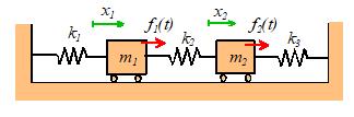
It is quite simple to find a formula for the motion of an undamped system subjected to time varying forces.   The predictions are a bit unsatisfactory, however, because their vibration of an undamped system always depends on the initial conditions.  In a real system, damping makes the steady-state response independent of the initial conditions.   However, we can get an approximate solution for lightly damped systems by finding the solution for an undamped system, and then neglecting the part of the solution that depends on initial conditions.

As an example, we will consider the system with two springs and masses shown in the picture.  Each mass is subjected to a harmonic force, which vibrates with some frequency $\omega$ (the forces acting on the different masses all vibrate at the same frequency). The equations of motion are

$\begin{array}{l}{m}_1\frac{d^2{x}_1}{d{t}^2}+\left(k_1+k_2\right)x_1-k_2{x}_2=F_1\cos \omega t\\ m_2\frac{d^2{x}_2}{d{t}^2}-k_2{x}_1+(k_2+k_3)x_2=F_2\cos \omega t\end{array}$

We can write these in matrix form as

$\left[\begin{array}{cc}{m}_1& 0\\ 0& m_2\end{array}\right]\frac{d^2}{d{t}^2}\left[\begin{array}{c}{x}_1\\ x_2\end{array}\right]+\left[\begin{array}{cc}{k}_1+k_2& -k_2\\ -k_2& k_2+k_3\end{array}\right]\left[\begin{array}{c}{x}_1\\ x_2\end{array}\right]=\left[\begin{array}{c}{F}_1\\ F_2\end{array}\right]$

or, more generally,

To find the steady-state solution, we simply assume that the masses will all vibrate harmonically at the same frequency as the forces.  This means that , , where  are the (unknown) amplitudes of vibration of the two masses.  In vector form we could write , where .  Substituting this into the equation of motion gives

This is a system of linear equations for X.  They can easily be solved using MATLAB.  As an example, here is a simple MATLAB function that will calculate the vibration amplitude for a linear system with many degrees of freedom, given the stiffness and mass matrices, and the vector of forces f.

function X = forced_vibration(K,M,f,omega)

% Function to calculate steady state amplitude of

% a forced linear system.

% K is nxn the stiffness matrix

% M is the nxn mass matrix

% f is the n dimensional force vector

% omega is the forcing frequency, in radians/sec.

% The function computes a vector X, giving the amplitude of

% each degree of freedom

%

X = (K-M*omega^2)\f;

end

The function is only one line long!

 

As an example, the graph below shows the predicted steady-state vibration amplitude for the spring-mass system, for the special case where the masses are all equal , and the springs all have the same stiffness .  The first mass is subjected to a harmonic force , and no force acts on the second mass.   Note that the graph shows the magnitude of the vibration amplitude $–$ the formula predicts that for some frequencies some masses have negative vibration amplitudes, but the negative sign has been ignored, as the negative sign just means that the mass vibrates out of phase with the force.

 

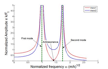
Several features of the result are worth noting:

       If the forcing frequency is close to any one of the natural frequencies of the system, huge vibration amplitudes occur.  This phenomenon is known as resonance.  You can check the natural frequencies of the system using the little matlab code in section 5.5.2 $–$ they turn out to be  and .  At these frequencies the vibration amplitude is theoretically infinite.

       The figure predicts an intriguing new phenomenon $–$ at a magic frequency, the amplitude of vibration of mass 1 (that’s the mass that the force acts on) drops to zero.   This is called ‘Anti-resonance,’ and it has an important engineering application.  Suppose that we have designed a system with a serious vibration problem (like the London Millenium bridge).  Usually, this occurs because some kind of unexpected force is exciting one of the vibration modes in the system.   We can idealize this behavior as a mass-spring system subjected to a force, as shown in the figure.  So how do we stop the system from vibrating?  Our solution for a 2DOF system shows that a system with two masses will have an anti-resonance.  So we simply turn our 1DOF system into a 2DOF system by adding another spring and a mass, and tune the stiffness and mass of the new elements so that the anti-resonance occurs at the appropriate frequency.   Of course, adding a mass will create a new vibration mode, but we can make sure that the new natural frequency is not at a bad frequency.   We can also add a dashpot in parallel with the spring, if we want $–$ this has the effect of making the anti-resonance phenomenon somewhat less effective (the vibration amplitude will be small, but finite, at the ‘magic’ frequency), but the new vibration modes will also have lower amplitudes at resonance. The added spring $–$ mass system is called a ‘tuned vibration absorber.’   This approach was used to solve the Millenium Bridge vibration problem.

 

 

5.6.5 The effects of damping

 

In most design calculations, we don’t worry about accounting for the effects of damping very accurately.  This is partly because it’s very difficult to find formulas that model damping realistically, and even more difficult to find values for the damping parameters.   Also, the mathematics required to solve damped problems is a bit messy. Old textbooks don’t cover it, because for practical purposes it is only possible to do the calculations using a computer.   It is not hard to account for the effects of damping, however, and it is helpful to have a sense of what its effect will be in a real system.  We’ll go through this rather briefly in this section.

 

Equations of motion: The figure shows a damped spring-mass system.  The equations of motion for the system can easily be shown to be

To solve these equations, we have to reduce them to a system that MATLAB can handle, by re-writing them as first order equations.  We follow the standard procedure to do this $–$ define  and  as new variables, and then write the equations in matrix form as

(This result might not be obvious to you $–$ if so, multiply out the vector-matrix products to see that the equations are all correct). This is a matrix equation of the form

where y is a vector containing the unknown velocities and positions of the mass.  

 

Free vibration response: Suppose that at time t=0 the system has initial positions and velocities , and we wish to calculate the subsequent motion of the system. To do this, we must solve the equation of motion. We start by guessing that the solution has the form  (the negative sign is introduced because we expect solutions to decay with time).  Here,  is a constant vector, to be determined.   Substituting this into the equation of motion gives

This is another generalized eigenvalue problem, and can easily be solved with MATLAB.  The solution is much more complicated for a damped system, however, because the possible values of  and  that satisfy the equation are in general complex $–$ that is to say, each  can be expressed as , where and are positive real numbers, and .  This makes more sense if we recall Euler’s formula

(if you haven’t seen Euler’s formula, try doing a Taylor expansion of both sides of the equation $–$ you will find they are magically equal.  If you don’t know how to do a Taylor expansion, you probably stopped reading this ages ago, but if you are still hanging in there, just trust me…).  So, the solution is predicting that the response may be oscillatory, as we would expect.  Once all the possible vectors  and  have been calculated, the response of the system can be calculated as follows:

1.      Construct a matrix H , in which each column is one of the possible values of  (MATLAB constructs this matrix automatically)

2.      Construct a diagonal matrix (t), which has the form

where each  is one of the solutions to the generalized eigenvalue equation.

3.      Calculate a vector a (this represents the amplitudes of the various modes in the vibration response) that satisfies

4.      The vibration response then follows as

All the matrices and vectors in these formulas are complex valued $–$ but all the imaginary parts magically disappear in the final answer.

 

HEALTH WARNING: The formulas listed here only work if all the generalized eigenvalues  satisfying are different.   For some very special choices of damping, some eigenvalues may be repeated.  In this case the formula won’t work.  A quick and dirty fix for this is just to change the damping very slightly, and the problem disappears.   Your applied math courses will hopefully show you a better fix, but we won’t worry about that here.

 

This all sounds a bit involved, but it actually only takes a few lines of MATLAB code to calculate the motion of any damped system. As an example, a MATLAB code that animates the motion of a damped spring-mass system shown in the figure (but with an arbitrary number of masses) can be downloaded here.   You can use the code to explore the behavior of the system.  In addition, you can modify the code to solve any linear free vibration problem by modifying the matrices M and D.

 

Here are some animations that illustrate the behavior of the system. The animations below show vibrations of the system with initial displacements corresponding to the three mode shapes of the undamped system (calculated using the procedure in Section 5.5.2).  The results are shown for k=m=1 . In each case, the graph plots the motion of the three masses $–$ if a color doesn’t show up, it means one of the other masses has the exact same displacement.

    

Mode 1                                           Mode 2                                          Mode 3

 

Notice that

1.      For each mode, the displacement history of any mass looks very similar to the behavior of a damped, 1DOF system.

2.      The amplitude of the high frequency modes die out much faster than the low frequency mode.

This explains why it is so helpful to understand the behavior of a 1DOF system.  If a more complicated system is set in motion, its response initially involves contributions from all its vibration modes.  Soon, however, the high frequency modes die out, and the dominant behavior is just caused by the lowest frequency mode. The animation to the right demonstrates this very nicely $–$ here, the system was started by displacing only the first mass.  The initial response is not harmonic, but after a short time the high frequency modes stop contributing, and the system behaves just like a 1DOF approximation.  For design purposes, idealizing the system as a 1DOF damped spring-mass system is usually sufficient.

 

Notice also that light damping has very little effect on the natural frequencies and mode shapes $–$ so the simple undamped approximation is a good way to calculate these.

 

Of course, if the system is very heavily damped, then its behavior changes completely $–$ the system no longer vibrates, and instead just moves gradually towards its equilibrium position.   You can simulate this behavior for yourself using the matlab code $–$ try running it with  or higher.   Systems of this kind are not of much practical interest.

 

 

 

 

 

 

 

Steady-state forced vibration response.  Finally, we take a look at the effects of damping on the response of a spring-mass system to harmonic forces.  The equations of motion for a damped, forced system are

 This is an equation of the form

where we have used Euler’s famous formula again.  We can find a solution to

by guessing that , and substituting into the matrix equation

This equation can be solved for.  Similarly, we can solve

by guessing that , which gives an equation for  of the form . You actually don’t need to solve this equation $–$ you can simply calculate  by just changing the sign of all the imaginary parts of . The full solution follows as

This is the steady-state vibration response.  Just as for the 1DOF system, the general solution also has a transient part, which depends on initial conditions. We know that the transient solution will die away, so we ignore it.

 

The solution for y(t) looks peculiar, because of the complex numbers.  If we just want to plot the solution as a function of time, we don’t have to worry about the complex numbers, because they magically disappear in the final answer.  In fact, if we use MATLAB to do the computations, we never even notice that the intermediate formulas involve complex numbers.  If we do plot the solution, it is obvious that each mass vibrates harmonically, at the same frequency as the force (this is obvious from the formula too).  It’s not worth plotting the function $–$ we are really only interested in the amplitude of vibration of each mass. This can be calculated as follows

1.      Let ,  denote the components of  and

2.      The vibration of the jth mass then has the form

where

are the amplitude and phase of the harmonic vibration of the mass.

If you know a lot about complex numbers you could try to derive these formulas for yourself.  If not, just trust me $–$ your math classes should cover this kind of thing.  MATLAB can handle all these computations effortlessly.  As an example, here is a simple MATLAB script that will calculate the steady-state amplitude of vibration and phase of each degree of freedom of a forced n degree of freedom system, given the force vector f, and the matrices M and D that describe the system.

function [amp,phase] = damped_forced_vibration(D,M,f,omega)

% Function to calculate steady state amplitude of

% a forced linear system.

% D is 2nx2n the stiffness/damping matrix

% M is the 2nx2n mass matrix

% f is the 2n dimensional force vector

% omega is the forcing frequency, in radians/sec.

% The function computes a vector ‘amp’, giving the amplitude of

% each degree of freedom, and a second vector ‘phase’,

% which gives the phase of each degree of freedom

%

Y0 = (D+M*i*omega)\f;  % The i here is sqrt(-1)

% We dont need to calculate Y0bar - we can just change the sign of

% the imaginary part of Y0 using the 'conj' command

for j =1:length(f)/2

    amp(j) = sqrt(Y0(j)*conj(Y0(j)));

    phase(j) = log(conj(Y0(j))/Y0(j))/(2*i);

end

end

Again, the script is very simple.

Here is a graph showing the predicted vibration amplitude of each mass in the system shown.  Note that only mass 1 is subjected to a force.

 

 

 

 

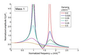
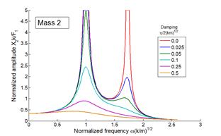
The important conclusions to be drawn from these results are:

1.      We observe two resonances, at frequencies very close to the undamped natural frequencies of the system.

2.      For light damping, the undamped model predicts the vibration amplitude quite accurately, except very close to the resonance itself (where the undamped model has an infinite vibration amplitude)

3.      In a damped system, the amplitude of the lowest frequency resonance is generally much greater than higher frequency modes.  For this reason, it is often sufficient to consider only the lowest frequency mode in design calculations.  This means we can idealize the system as just a single DOF system, and think of it as a simple spring-mass system as described in the early part of this chapter.  The relative vibration amplitudes of the various resonances do depend to some extent on the nature of the force $–$ it is possible to choose a set of forces that will excite only a high frequency mode, in which case the amplitude of this special excited mode will exceed all the others.   But for most forcing, the lowest frequency one is the one that matters.

4.      The ‘anti-resonance’ behavior shown by the forced mass disappears if the damping is too high.