Diffusion Tensor Imaging (DTI)
This example provides a single example for a ROI-based method of analyzing diffusion tensor imaging data using FSL, TORTOISE, and AFNI.
Remember: there are many ways to analyze DTI data that may be better suited to your needs. This is just one example.
Prior to beginning this analysis, you will need to install FSL, TORTOISE, and AFNI on your computer. These programs can be downloaded on the following sites:
We also assume you are familiar with UNIX or shell scripting. If not, visit AFNI's Unix Tutorial before beginning this analysis.
You can follow along with our analysis steps using our example dataset. If you do not wish to use the example dataset, be certain to change the names of the files in the below examples to correspond to the dataset you are using.
Note that this example is for a single subject and a single ROI, so we provide specific commands to run rather than a script for processing multiple subjects. It would be helpful to create your own script using these commands for use with multiple subjects and ROIs.
Contents:
- Step 1: Prepare T1 image for use in TORTOISE
- Step 2: Processing with TORTOISE
- Step 3: Calculate tensors
- Step 4: MNI transform
- Step 5: Create ROIs
- Step 6: Extract FA/MD/RD values from ROIs
- Step 7: Statistical analysis
- Additional Resources
Step 1: Prepare T1 image for use in TORTOISE
The bulk of our DTI analysis will involve the NIH's open source program TORTOISE.
BUT, before we use TORTOISE, we need to prepare our anatomical image for use in this program.
It is recommended that you use a T2-weighted anatomical image in TORTOISE because it has similar characteristics to diffusion data. However, we are using a T1-weighted image for this tutorial because we did not collect a T2 image for this dataset.
Through consulation with a TORTOISE developer, we came up with a way to utilize a T1 image when lacking a T2. This involves separating brain and non-brain regions, attenuating the non-brain regions, and then putting the brain regions back together with the attenuated non-brain regions to produce a final attenuated-T1.
If you are using a T2 image rather than following along with our example dataset, you can skip the following steps below and proceed with Step 2.
Otherwise, perform the following steps to produce an attenuated-T1 image for use with TORTOISE.
First, we will use FSL's fslreorient2std command to re-orient our anatomical image to the orientation of the MNI152 standard template. To do so, run the following command for each participant's T1 image:
fslreorient2std s01_T1.nii s01_T1_std.nii
Next, we will remove non-brain tissue from our T1 image using FSL's BET tool by running the following command for each participant's T1 image:
bet s01_T1_std.nii s01_T1_bet.nii.gz -B -f 0.4 -g 0
NOTE: This step will take ~10 mins-15**
Then, we will attenuate the non-brain regions of the T1 and add the attenuated non-brain regions back to the brain regions to produce a final attenuated-T1. To do so, run the following command:
fslmaths s01_T1_std.nii -sub s01_T1_bet.nii.gz -div 10 -add s01_T1_bet.nii.gz s01_T1_att.nii
NOTE: This will create a zipped file named s01_T1_att.nii.gz. Before continuing on with the next steps, unzip this file by typing this command: gunzip s01_T1_att.nii.gz
Step 2: Processing with TORTOISE
The bulk of processing for this analysis will be done using TORTOISE. For more information on the program, visit the NIH's webpage for this program.
Once you have downloaded the program (following directions from link at top of page), continue with the next steps.
TORTOISE has two main components, DIFF_PREP, which handles pre-processing of the diffusion images, and DIFF_CALC, which handles the calculations.
Step 2a: DIFF_PREP
Once you have downloaded TORTOISE, the downloaded program folder (TORTOISE_V2.5.1, or corresponding version) will contain several subfolders.
Within the TORTOISE_V2.5.1 folder, click on the DIFF_PREP subfolder, and then the diffprep_main subfolder.
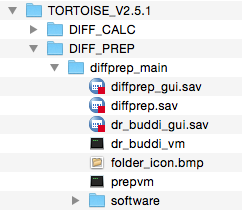
From there, you should see the prepvm executable file. Double-click on prepvm, which will launch Terminal.
Click "OK" on the IDL Virtual Machine GUI that launches automatically, which will open the DIFF_PREP GUI and the Registration Status Report Window.
Before continuing further with DIFF_PREP, it may be helpful to first browse through the DIFF_PREP Software Guide.
Using the DIFF_PREP GUI, perform the following steps:
Left side of GUI:
- Input data format: FSL 4D NIFTI file (select this option because we prepared our files using FSL in step 1 above)
- FSL NIFTI file path: navigate to the diffusion image file (s01_DTI.nii)
- Make sure that the folder containing this file also contains the corresponding bvec and bval files
- Tortoise will search sub-folders for these files, so make sure you do not have multiple bvec or bval files in this folder or in any sub-folders or you will get an error
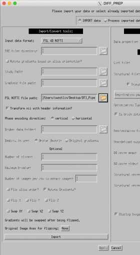
- Click on "import" at the left bottom of the GUI
To make sure this step ran successfully, check the Registration Status Report Window.
The window should print the following message:
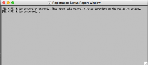
This will generate a folder named s01_DTI_proc in the same directory as the folder containing your s01_DTI.nii file.
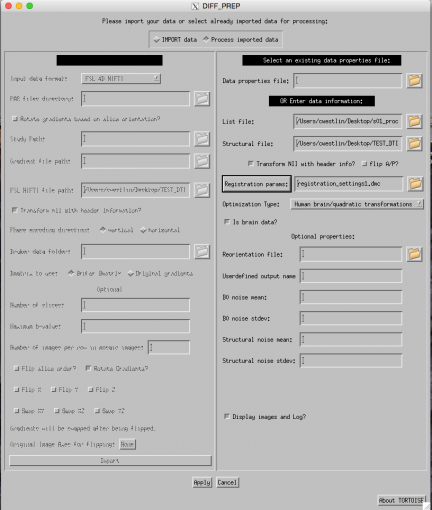
Once you import these files, perform the following steps:
Right side of GUI:
- List file: navigate to the s01_DTI_proc folder generated in the step above, and click on the .list file
- Structural file: navigate to the modified T1 image we created in Step 1 (s01_T1_att.nii)
- Registration params: click on the registration params button to open the registration settings page. Leave everything as default, other than the following changes:
- LEFT SIDE:
- ITK Structural registration: OFF
- RIGHT SIDE:
- Quadratic correction for subsequent B0s: OFF
- Keep intermediate data: OFF
NOTE for Correction for B0 distortion with BSplines option:
It is recommended that a fat saturated T2-weighted structural image be provided for the EPI distortion correction to work appropriately. The contrast between the structures on the T2 image lends itself to better EPI correction results. If T2 image is unavailable, EPI correction with T1-weighted image can be attempted but we have not seen good results. Thus, when using a T1 or related contrast structural image, switch OFF the EPI correction option. We are using a T1 attenuated skull-stripped image, BUT will keep this ON just to see if it might work.Your final Registration Settings GUI should look like this – make sure all parameters are as seen in this image:
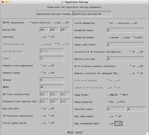
- LEFT SIDE:
- Click "Apply" at the bottom of the GUI, which will create a registration_settings1.dmc file located in your home directory ~/DIFF_PREP_WORK
Make sure that this newly created file is selected under the Registration params option of the DIFF_PREP GUI
- Click "Apply" at the bottom of the GUI – this will take about 4 hours per dataset. To make sure it is running successfully and you are not encountering any errors, view the status of the processing in the Registration Status Report Window.
Your final GUI before pressing apply should look similar to this:
If you are following this tutorial using our sample dataset simply to learn the process, we have provided the files that result from the DIFF_PREP steps above so that you do not have to wait the 4 hours for this step to run.
You will know this process is finished when "[Process completed]" is printed in the terminal window.
Step 2b: DIFF_CALC
After successfully pre_processing via DIFF_PREP, we will now use DIFF_CALC to inspect the results of DIFF_PREP and export the data to AFNI.
Before beginning this process, it may be helpful to browse through the DIFF_CALC Software Guide.
As in Step 2a, open the program folder (TORTOISE_V2.5.1, or corresponding version) which contains several subfolders.
Within the TORTOISE_V2.5.1 folder, click on the DIFF_CALC subfolder, and then the diffcalc_main subfolder.
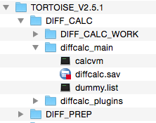
From there, you should see the calcvm executable file. Double-click on calcvm, which will launch Terminal.
Click "OK" on the IDL Virtual Machine GUI that launches automatically, which will open the DIFF_CALC GUI and the Status Report Window.
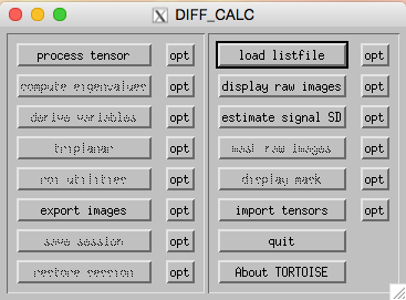
Using the DIFF_CALC GUI, perform the following steps:
- Load listfile (right side of GUI): navigate to the s01_DTI_proc folder that was created by the DIFF_PREP steps, then choose the .list file (s01_DTI.list)
- Display raw images (right side of GUI): click on this to inspect the raw data
NOTE: Tortoise provides a helpful guide to displaying images
You can use the scroll bar under "SLICES" to scroll through each slice and inspect the images to ensure there are no artifacts. You can also click the "INSPECT ENTIRE SET" button to view all slices at once.
- "Delete volume" button at bottom of raw images GUI
After visual inspection, delete any volumes containing artifacts, etc. We will not be deleting any volumes as part of this tutorial, but feel free to play around with the data as you please.
NOTE: Make sure to add one to the volume number from FSL when removing volumes in DIFF_CALC
NOTE: Remove volumes with higher numbers first – e.g., if you are removing volume 34 and volume 21, make sure to remove 34 first and then 21
- When you have removed all volumes that you needed to, click "DONE"-- this will create a new list file with the addition of _DR to the file name (s01_DTI_30dir_4D_DR.list)
- Go back to the "load listfile" button and select the new _DR.list file you just created
NOTE: Double check the number of volumes to confirm that this number matches the number of remaining volumes you expect after deletion of volumes with artifacts
Because we are not deleting any volumes as part of this tutorial, you may use the original .list file. But be certain to use the _DR.list file if you decided to delete any volumes for your dataset.
- "Delete volume" button at bottom of raw images GUI
- Export images (left side f GUI): select AFNI (may take a few minutes to export), then click "DONE"
Step 3: Calculate tensors
After performing the above steps, we will then calculate tensors using AFNI. Prior to this step, you will need to copy files generated from previous steps into a new directory. You will need the following files:
- The pre-processed DWI file
This file is located within the s01_DTI_proc folder, in a subfolder titled s01_DTI_SAVE_AFNI. It should be called "DWI.nii"
- BMTXT.txt file
This file is located in the same folder as the DWI.nii file above
- The registered structural image
This file is located within the s01_DTI_proc folder. It should be called s01_DTI_DMCstructural.nii
After saving these three images into a new directory, you are ready to begin tensor calculations using AFNI.
First, you will need to skull strip the structural image. To do so, enter the following command in terminal (this step will take ~10 minutes).
NOTE: Make sure you navigate to the correct directory in yor terminal that contains the three files above before entering this command
3dSkullStrip -input s01_DTI_DMCstructural.nii -prefix s01_structural_ns.nii -push_to_edge -blur_fwhm 2 -shrink_fac 0.4 -avoid_vent -avoid_vent -niter 400 -ld 40
Then, we will create a brain mask of this skull-stripped structural image. To do so, run the following command:
3dcalc -a s01_structural_ns.nii -expr 'ispositive(a)' -prefix s01_brainmask.nii -float
Now we are ready to calculate tensors. To do this, enter the following command:
3dDWItoDT -echo_edu \
    -prefix s01.nii \
    -mask s01_brainmask.nii \
    -eigs -sep_dsets -nonlinear \
    -bmatrix_Z BMTXT.txt DWI.nii \
    -overwrite
Note: if you get an error that the mask and input datasets are not the same size, you may need to resample your mask to match the DWI.nii dataset using 3dresample
Running the above command will result in the creation of DT, FA, L1, L2, L3, MD, V1, V2, and V3 files. If you would also like to create a RD file, enter the following command:
3dcalc -a s01_L2.nii -b s01_L3.nii -prefix s01_RD.nii -expr '(a+b)/2'
Step 4: MNI transform
After creating the tensors in AFNI, we want to convert the FA, MD, and RD images into standard space so that we can utilize a brain atlas for ROI selection.
We will first convert the FA image to MNI standard space using FSL's FLIRT and FNIRT tools.
To do this, we will utilize the FMRIB58_FA_1mm.nii.gz image contained within the fsl/data/standard/ directory. For ease of use in this tutorial, we have also included this image file in our tutorial download folder.
Copy the FMRIB58_FA_1mm.nii.gz image into the same directory as the tensor files calculated in the step above, and then run the following FLIRT command:
flirt -in s01_FA.nii -ref FMRIB58_FA_1mm.nii.gz -out s01_FA_flirt -omat s01_FA_flirt.mat -bins 256 -cost corratio -searchrx -90 90 -searchry -90 90 -searchrz -90 90 -dof 12 -interp trilinear
Then, run the following FNIRT command:
fnirt --ref=FMRIB58_FA_1mm.nii.gz --in=s01_FA --aff=s01_FA_flirt.mat --cout=s01_FA_fnirt_transf --config=FA_2_FMRIB58_1mm
We will then apply the fnirt transformatin matrix created by the command above to the s01_FA.nii, s01_MD.nii, and s01_RD.nii images by entering the following commands, one at a time:
applywarp --ref=FMRIB58_FA_1mm.nii.gz --in=s01_FA --warp=s01_FA_fnirt_transf --out=s01_FA_fnirt
applywarp --ref=FMRIB58_FA_1mm.nii.gz --in=s01_MD --warp=s01_FA_fnirt_transf --out=s01_MD_fnirt
applywarp --ref=FMRIB58_FA_1mm.nii.gz --in=s01_RD --warp=s01_FA_fnirt_transf --out=s01_RD_fnirt
Step 5: Create ROIs
After converting the FA, MD, and RD images to MNI158 standard space, we then need to select the ROIs that we will be using to analyze these images.
There are many different ways to create ROIs, but we will be using an atlas-based method.
We will be using FSL's JHU White Matter Tractography Atlas. This atlas is located in the FSL directory under /usr/local/fsl/data/atlases/
If you are unsure of FSL's location on your computer, type "which fsl" in the command line. This will tell you the location of the folder, within which the /data/atlases/ folders will be.
There is a list of available regions and corresponding atlas codes in the atlases folder (JHU-labels.xml and JHU-tracts.xml). This folder also contains a sub-folder, JHU, which contains the atlas we will be using (JHU-ICBM-labels-1mm.nii.gz). Copy this atlas into the directory containing the FA/MD/RD images.
For our example, we will be using the splenium as our ROI (atlas code "5").
To create the splenium ROI, enter the following command:
fslmaths JHU-ICBM-labels-1mm.nii.gz -thr 5 -uthr 5 Splenium.nii
We then need to binarize the mask so that the ROI mask has a value of "1" and all other areas have a value of "0". Do this by running the following command:
fslmaths Splenium.nii -bin Splenium_binarized.nii
Step 6: Extract FA/MD/RD values from ROIs
Once we have our ROI mask created, we then need to extract the values from within that ROI for the FA/MD/RD images.
First, you need to multiply the binarized ROI mask by the FA/MD/RD image
NOTE: Our example from here on will only do this for FA, but repeat the same steps for MD and RD
To do this, run the following command:
fslmaths s01_FA_fnirt.nii.gz -mul Splenium_binarized.nii.gz s01_FA_Splenium
Then, extract whatever values you may wish to extract from that image. We will be extracting the mean and standard deviation by running the following command:
fslstats s01_FA_Splenium -M -S
The above command will output two values, the mean being the first value (specified by -M) and the SD being the second (-S option). If you wish to write these values to a text file, you may want to enter a variation of the following command:
fslstats s01_FA_Splenium -M -S | tee -a Splenium_output.txt
Step 7: Statistical analysis
Once you have extracted all values of interest from every participant and ROI, you may run whichever statistics you wish to perform on your data.
Additional Resources
Our example provides only one method of conducting a ROI-based method of analyzing diffusion tensor data.
However, there are many other methods to do this type of analysis, and there are many resources available online explaining alternative methods.
Below we provide a few resources to enhance your understanding of DTI analysis.
A great resource for imaging analyses is Andy's Brain Blog. He provides a series of videos on DTI analyses.
This CogNeuroStats Blog provides a very helpful overview of DTI processing using TORTOISE, broken into two parts. Part 1 provides an overview of DIFF_PREP while Part 2 provides an overview of DIFF_CALC.
The Human Connectome Project also provides an overview of Diffusion Tractography.