Resting State fMRI Analysis
This example provides a ROI-based method of analyzing resting state fMRI data using AFNI.
Prior to beginning this analysis, you will need to install AFNI on your computer. AFNI's Installation Guide provides detailed information on how to download the program.
If you are unfamiliar with UNIX or shell scripting, visit AFNI's Unix Tutorial before beginning this analysis.
You can follow along with our analysis steps using our example dataset. If you do not wish to use the example dataset, be certain to change the names of the files in the below examples to correspond to the dataset you are using.
Note that this example is for a single subject and a single ROI, so we provide specific commands to run rather than a script for processing multiple subjects.
It would be helpful to create your own script using these commands for use with multiple subjects and ROIs.
Contents:
- Step 1: Pre-processing
- Step 2: Create ROIs
- Step 3: Create correlation maps
- Step 4: Group analyses
- Additional Resources
Step 1: Pre-processing
To pre-process resting state fMRI data, we use AFNI's processing stream afni_proc.py (example 9b). For more information, visit the afni_proc.py program help page.
AFNI also provides a graphical interface for afni_proc.py via a program called uber_subject.py. For more information, visit the uber_subject.py program help page. Andy's Brain Blog also provides a helpful video on how to use this program for resting state analysis. For more information on this blog, see the Additional Resources section of this page.
Inputs to afni_proc.py:
-anatomical dataset (s01_anat.nii)
-resting state EPI time series dataset (s01_rest_EPI.nii)
To pre-process the data using afni_proc.py, run the following command for each participant:
afni_proc.py -subj_id s01.REST \
	-dsets s01_rest_EPI.nii \
	-copy_anat s01_anat.nii \
	-blocks despike tshift align tlrc volreg blur mask regress \
	-tcat_remove_first_trs 3 \
	-volreg_align_e2a \
	-volreg_tlrc_warp \
	-regress_anaticor \
	-regress_censor_motion 0.2 \
	-regress_censor_outliers 0.1 \
	-regress_bandpass 0.01 0.1 \
	-regress_apply_mot_types demean deriv \
	-regress_run_clustsim no \
	-regress_est_blur_epits \
	-regress_est_blur_errts
Running the above command will generate a script (proc.s01.REST). You will need to run this script in your command line to complete pre-processing. This is the longest step (takes ~20-30 minutes if you are running this locally on your computer).
To run this script, AFNI suggests the following commands:
- if you use tcsh: tcsh -xef SCRIPT |& tee output.SCRIPT
- if you use bash: tcsh -xef SCRIPT 2>&1 | tee output.SCRIPT
Running this script will generate a folder containing the results (s01.REST.results). The dataset of interest within that folder is the errts dataset (errts.s01.REST.anaticor+tlrc).
Note that we are using the default AFNI parameters for afni_proc.py resting state example 9b. These can be changed based on individual needs of your dataset (see the afni_proc.py help page).
Below is a brief description of each option in the above afni_proc.py command:
- -subj_id
- creates a label for the output of this processing step
- -dsets
- input resting state EPI dataset to be processed
- -copy_anat
- makes a copy of your anatomical dataset to store in output directory
- -blocks
- outlines specific pre-processing steps that will be done
- -tcat_remove_first_trs
- removes number of specified volumes from beginning of functional scan (in this case, we specify that the first 3 be removed)
- -volreg_align_e2a
- aligns EPI to anat
- -volreg_tlrc_warp
- warps to standard Talairach space
- -regress_anaticor
- generates error time series (errts dataset) using ANATICOR method (see ANATICOR help for more information)
- -regress_censor_motion
- provides motion limit for TRs that will be removed (we use estimate of 0.2, which is more conservative than task-based analyses to minimize effects of head motion)
- -regress_censor_outliers
- censors TRs when more than 10% of the automasked brain are outliers (using 0.1 option)
- -regress_bandpass
- performs bandpass filtering during the linear regression (using lower and upper frequency limits of 0.01 0.1)
- -regress_apply_mot_types
- include both de-meaned and derivatives of motion parameters in the regression
- -regress_run_clustsim
- controls whether 3dClustSim will be executed after regression analysis for use in multiple comparison correction (we do not need this option so used "no" option)
- -regress_est_blur_epits
- estimates the smoothness of the EPI data
- -regress_est_blur_errts
- estimates the smoothness of the error time series (errts)
Step 2: Create ROIs
To conduct a ROI-based analysis examining connectivity between seed regions and all other brain voxels, we first need to create the ROI(s) of interest.
There are several methods that can be used to create ROIs: hand-drawn, atlas-based, etc.
AFNI provides a helpful handout for understanding how to create ROIs.
Our example will use the built-in AFNI TT_Daemon atlas.
To see all regions available in AFNI's built-in atlases, type the following command:
whereami -show_atlas_code | less
(To scroll through this list of atlases and corresponding regions, press return key to display each subsequent line. To quit out of this view, press "q")
You will need the atlas code for each region you want to include in your analysis.
For our example, we will be using the left amygdala as our ROI (TT_Daemon atlas code 271).
To generate a mask of this ROI, type the following command (using L Amyg example):
whereami -mask_atlas_region TT_Daemon:271 -prefix LAmyg.nii
NOTE: If you receive a "no exact match for 271" error, try repacing TT_Daemon:271 with TT_Daemon:left:Amygdala
Before continuing, make sure the LAmyg.nii mask you just generated is in the same directory as the errts dataset generated in step 1.
Then, resample the mask you just created so that its grid spacing matches that of the errts dataset:
3dresample -master errts.s01.REST.anaticor+tlrc -inset LAmyg.nii -prefix LAmyg_resampled.nii
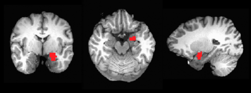
The left amygdala ROI you create, overlayed on the anatomical image, should look like the image below:
Step 3: Create correlation maps
Step 3a: Extract mean time series within each ROI
To extract mean time series within each ROI, we will use AFNI's 3dROIstats command.
Run the following command for each participant, for each ROI:
3dROIstats -mask LAmyg_resampled.nii -1Dformat errts.s01.REST.anaticor+tlrc > s01_LAmyg.1D
Step 3b: Generate Pearson correlation between mean time series and all other voxels
To generate a Pearson correlation between the mean time series within each ROI and all other voxels, we will use AFNI's 3dTcorr1D command.
Run the following command for each participant, for each ROI:
3dTcorr1D -pearson -prefix s01_LAmyg.Tcorr1D.nii errts.s01.REST.anaticor+tlrc s01_LAmyg.1D
Step 3c: Convert r score to a z score for use in group analyses
To convert each r score to a z score, we will use AFNI's 3dcalc command.
Run the following command for each participant, for each ROI:
3dcalc -a s01_LAmyg.Tcorr1D.nii -expr 'atanh(a)' -prefix s01_LAmyg.z.nii
The z score image, thresholded and overlayed on the anatomical image, should look similar to the image below:
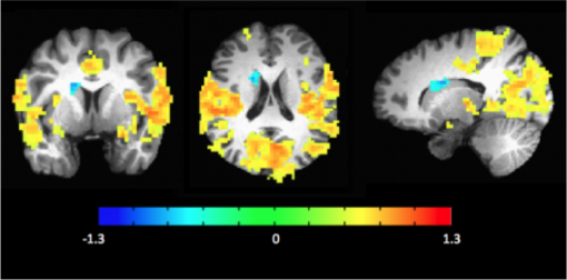
If you find that many voxels are active outside the brain volume for your data, it may be useful to mask the brain first to avoid this.
Step 4: Group analyses
After running Steps 1-3 on all subjects and ROIs relevant to your study, perform the analysis that is best fit to your design using the .z files created in Step 3c.
If you are unsure of the best group analysis to run for your data, AFNI's group analysis guide may be a good place to start. Common group analysis programs are 3dttest and 3dANOVA.
Andy's Brian Blog provides an example of a second level group analysis using AFNI's uber_ttest.py.
AFNI's statistics guru Gang Chen also has a website which may be helpful in understanding which statistics you should run for your study.
Additional Resources
Our example provides only one method of conducting a seed-based resting state functional connectivity analysis.
However, there are many other methods to do this type of analysis, and there are many resources available online explaining alternative methods.
Below we provide a few resources to enhance your understanding of resting state analysis.
A great resource for imaging analyses is Andy's Brain Blog. He provides a series of videos on resting state analyses. His analysis uses slightly different analysis steps, but it is a valuable resource for anyone trying to learn the basics of resting state functional connectivity analysis.
AFNI also provides guides to connectivity analysis and resting state analysis to help you better understand resting state connectivity analysis.
The Human Connectome Project also provides an overview of resting state fMRI.